Creating fusion source with AFSI
This example shows how to create a fusion source with AFSI in various cases.
AFSI (Ascot Fusion Source Integrator) calculates the 5D distributions of fusion reaction products based on the 5D distributions of the reactants. The algorithm iterates over all cells in cylindrical coordinates, and on each location creates fusion products via Monte Carlo sampling. First, a pair of markers is sampled from the reactant (velocity) distributions and the velocities of the fusion products for a given reaction are calculated using the initial velocities. The reaction probability, which depends on the relative velocity between the reactants, is used to weight the products which in turn are used to calculate the 5D distributions for the output. Several pairs are created before the algorithm proceeds to the next cylindrical cell.
The Monte Carlo sampling makes AFSI capable of not only calculating reactions for thermal (Maxwellian) species but for arbitrary distributions. In practice this often means NBI slowing-down distributions and, hence, the arbitrary distribution is referred to as beam when working with AFSI.
Note that AFSI calculates the distributions for both products, i.e., one can use AFSI to calculate the neutron source as well.
AFSI has three modes of operation based on what the inputs are:
thermalcalculates the fusion products for two Maxwellian species. The population can also react itself as is the case with D-D fusion.beam-thermalcalculates the fusion products for a Maxwellian species that is interacting with an arbitrary distribution.beam-beamcalculates the fusion products for two arbitrary distributions. A distribution can interact with itself, e.g. if there is a single deuterium beam.
AFSI requires only the magnetic field and plasma data for it to work, but we also need to get the beam ion distribution somewhere for this tutorial. The following cell initializes the inputs and runs a short slowing-down simulation for a deuterium beam. Its contents are not relevant for this tutorial.
[1]:
import numpy as np
import matplotlib.pyplot as plt
from a5py import Ascot

a5 = Ascot("ascot.h5", create=True)

a5.data.create_input("bfield analytical iter circular", desc="ANALYTICAL")

# DT-plasma
nrho  = 101
rho   = np.linspace(0, 2, nrho).T
prof  = (rho<=1)*(1.0 - rho**(3.0/2))**3 + 1e-6
vtor  = np.zeros((nrho, 1))
edens = 2e21 * prof
etemp = 1e4  * np.ones((nrho, 1))
idens = 1e21 * np.tile(prof,(2,1)).T
itemp = 1e4  * np.ones((nrho, 1))

edens[rho>=1]   = 1
idens[rho>=1,:] = 1

pls = {
    "nrho" : nrho, "nion" : 2, "rho" : rho, "vtor": vtor,
    "anum" : np.array([2, 3]), "znum" : np.array([1, 1]),
    "mass" : np.array([2.014, 3.016]), "charge" : np.array([1, 1]),
    "edensity" : edens, "etemperature" : etemp,
    "idensity" : idens, "itemperature" : itemp}
a5.data.create_input("plasma_1D", **pls, desc="DT")

# These inputs are not relevant for AFSI
a5.data.create_input("wall rectangular")
a5.data.create_input("E_TC")
a5.data.create_input("N0_1D")
a5.data.create_input("Boozer")
a5.data.create_input("MHD_STAT")
a5.data.create_input("asigma_loc")

# Generate deuterium markers with Ekin=1MeV and run a short slowing down simulation.
from a5py.ascot5io.marker import Marker
mrk = Marker.generate("gc", n=100, species="deuterium")
mrk["energy"][:] = 1.0e6
mrk["pitch"][:]  = 0.99 - 0.2 * np.random.rand(100,)
mrk["r"][:]      = np.linspace(6.2, 7.2, 100)
a5.data.create_input("gc", **mrk)

from a5py.ascot5io.options import Opt
opt = Opt.get_default()
opt.update({
    "SIM_MODE":2, "ENABLE_ADAPTIVE":1,
    "ENDCOND_SIMTIMELIM":1, "ENDCOND_MAX_MILEAGE":0.05,
    "ENABLE_ORBIT_FOLLOWING":1, "ENABLE_COULOMB_COLLISIONS":1,
    "ENABLE_DIST_5D":1,
    "DIST_MIN_R":4.3,        "DIST_MAX_R":8.3,       "DIST_NBIN_R":50,
    "DIST_MIN_PHI":0,        "DIST_MAX_PHI":360,     "DIST_NBIN_PHI":1,
    "DIST_MIN_Z":-2.0,       "DIST_MAX_Z":2.0,       "DIST_NBIN_Z":50,
    "DIST_MIN_PPA":-1.3e-19, "DIST_MAX_PPA":1.3e-19, "DIST_NBIN_PPA":100,
    "DIST_MIN_PPE":0,        "DIST_MAX_PPE":1.3e-19, "DIST_NBIN_PPE":50,
    "DIST_MIN_TIME":0,       "DIST_MAX_TIME":1.0,    "DIST_NBIN_TIME":1,
    "DIST_MIN_CHARGE":1,     "DIST_MAX_CHARGE":3,    "DIST_NBIN_CHARGE":1,
})
a5.data.create_input("opt", **opt, desc="SLOWINGDOWN")

import subprocess
subprocess.run(["./../../build/ascot5_main", "--d=\"BEAMSD\""])
print("Simulation complete")
/home/runner/work/ascot5/ascot5/a5py/routines/plotting.py:35: UserWarning: Could not import cKDTree and alphashape. 3D surface plotting disabled.
  warnings.warn(
ASCOT5_MAIN
Tag 6290a22
Branch docs

Initialized MPI, rank 0, size 1.

Reading and initializing input.

Input file is ascot.h5.

Reading options input.
Active QID is 1214415972
Options read and initialized.

Reading magnetic field input.
Active QID is 3104489752

Analytical tokamak magnetic field (B_GS)
Psi at magnetic axis (6.618 m, -0.000 m)
-5.410 (evaluated)
-5.410 (given)
Magnetic field on axis:
B_R = 0.000 B_phi = 4.965 B_z = -0.000
Number of toroidal field coils 0
Magnetic field read and initialized.

Reading electric field input.
Active QID is 2586455633

Trivial Cartesian electric field (E_TC)
E_x = 0.000000e+00, E_y = 0.000000e+00, E_z = 0.000000e+00
Electric field read and initialized.

Reading plasma input.
Active QID is 1614721122

1D plasma profiles (P_1D)
Min rho = 0.00e+00, Max rho = 2.00e+00, Number of rho grid points = 101, Number of ion species = 2
Species Z/A  charge [e]/mass [amu] Density [m^-3] at Min/Max rho    Temperature [eV] at Min/Max rho
   1  /  2     1  /  2.014             1.00e+21/1.00e+00                1.00e+04/1.00e+04
   1  /  3     1  /  3.016             1.00e+21/1.00e+00                1.00e+04/1.00e+04
[electrons]   -1  /  0.001             2.00e+21/1.00e+00                1.00e+04/1.00e+04
Toroidal rotation [rad/s] at Min/Max rho: 0.00e+00/0.00e+00
Quasi-neutrality is (electron / ion charge density) 2.00
Toroidal rotation [rad/s] at Min/Max rho: 0.00e+00/0.00e+00
Plasma data read and initialized.

Reading neutral input.
Active QID is 3609474777

1D neutral density and temperature (N0_1D)
Grid:  nrho =    3   rhomin = 0.000   rhomax = 2.000
 Number of neutral species = 1
Species Z/A   (Maxwellian)
        1/  1 (1)
Neutral data read and initialized.

Reading wall input.
Active QID is 0637300694

2D wall model (wall_2D)
Number of wall elements = 20, R extend = [4.10, 8.40], z extend = [-3.90, 3.90]
Wall data read and initialized.

Reading boozer input.
Active QID is 4198425967

Boozer input
psi grid: n =    6 min = 0.000 max = 1.000
thetageo grid: n =   18
thetabzr grid: n =   10
Boozer data read and initialized.

Reading MHD input.
Active QID is 2212345775

MHD (stationary) input
Grid: nrho =    6 rhomin = 0.000 rhomax = 1.000

Modes:
(n,m) = ( 1, 3) Amplitude = 0.1 Frequency =   1 Phase =   0
(n,m) = ( 2, 4) Amplitude =   2 Frequency = 1.5 Phase = 0.785
MHD data read and initialized.

Reading atomic reaction input.
Active QID is 3662209399

Found data for 1 atomic reactions:
Reaction number / Total number of reactions = 1 / 1
  Reactant species Z_1 / A_1, Z_2 / A_2     = 0 / 0, 0 / 0
  Min/Max energy                            = 1.00e+03 / 1.00e+04
  Min/Max density                           = 1.00e+18 / 1.00e+20
  Min/Max temperature                       = 1.00e+03 / 1.00e+04
  Number of energy grid points              = 3
  Number of density grid points             = 4
  Number of temperature grid points         = 5
Atomic reaction data read and initialized.

Reading marker input.
Active QID is 0855568251

Loaded 100 guiding centers.
Marker data read and initialized.

All input read and initialized.

Initializing marker states.
Estimated memory usage 0.0 MB.
Marker states initialized.

Preparing output.
Note: Output file ascot.h5 is already present.

The qid of this run is 0744233918

Inistate written.
Simulation begins; 4 threads.
Simulation complete.
Simulation finished in 10.646592 s
Endstate written.

Combining and writing diagnostics.

Writing diagnostics output.

Writing 5D distribution.

Diagnostics output written.
Diagnostics written.

Summary of results:
      100 markers had end condition Sim time limit

          No markers were aborted.

Done.
Simulation complete
AFSI is used via the Ascot object using the attribute afsi which has all the relevant methods. To use AFSI, we need to specify what reaction is that we are considering. To list possible reactions:
[2]:
a5.afsi.reactions()
[2]:
dict_keys(['DT_He4n', 'DHe3_He4p', 'DD_Tp', 'DD_He3n'])
To run AFSI on thermal mode, we need to specify \((R,z)\), and optionally \(\phi\), grid on which the distributions are calculated. Since both reactant populations are Maxwellian, there is no need to define velocity grids for those as AFSI can use the analytical distribution. Specifying the velocity grid for the products is required however.
Once inputs are set, we can call thermal function that computes the product distributions for us.
[3]:
# Grid spanning the whole plasma
r = np.linspace(4.2, 8.2, 51)
z = np.linspace(-2.0, 2.0, 51)
ppar = np.linspace(-1.3e-19, 1.3e-19, 81)
pperp = np.linspace(0, 1.3e-19, 41)

# Run AFSI which creates a fusion alpha distribution
a5.afsi.thermal(
    "DT_He4n", nmc=1000, r=r, z=z,
    ppar1=ppar, pperp1=pperp, ppar2=ppar, pperp2=pperp
    )
[3]:
(<a5py.ascotpy.ascot2py.struct_histogram at 0x7ff360eacfc0>,
 <a5py.ascotpy.ascot2py.struct_histogram at 0x7ff360ead7c0>)
The result is stored in the HDF5 file in a similar run group (found in a5.data) as the ASCOT5 simulations are, and the group works in a similar manner. The group contains information on the magnetic field and plasma inputs that were used and provides methods to access the product distributions. However, now the distributions are called prod1 and prod2 instead of 5d, but they act exactly as a 5d distribution would.
[4]:
alphadist = a5.data.active.getdist("prod1")
alphadist.integrate(time=np.s_[:], charge=np.s_[:]) # Distribution must be 5D

rzdist  = alphadist.integrate(copy=True, phi=np.s_[:], ppar=np.s_[:], pperp=np.s_[:])
momdist = alphadist.integrate(copy=True, phi=np.s_[:], r=np.s_[:], z=np.s_[:])

fig = plt.figure(figsize=(10,5))
ax1 = fig.add_subplot(1,2,1)
ax2 = fig.add_subplot(1,2,2)

rzdist.plot(axes=ax1)
momdist.plot(axes=ax2)

plt.show()
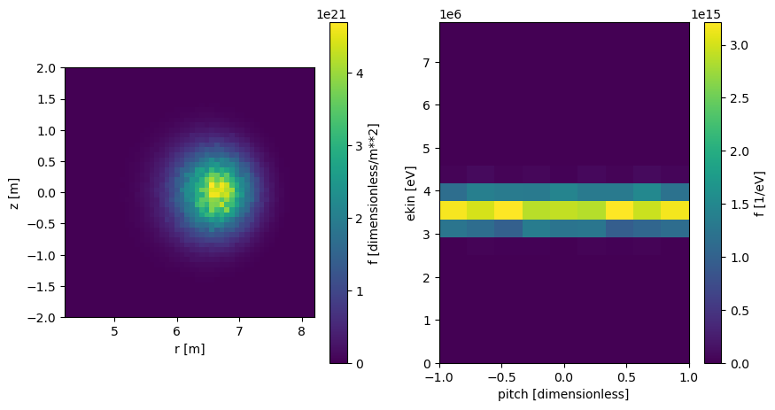
The momentum space can either be \((p_\parallel,p_\perp)\) or \((E_\mathrm{kin},\xi=p_\parallel/p)\). While the spatial grid must be the same for both products, the momentum grid can be different as long as the basis is the same. Here’s the thermal fusion calculation redone using energy-pitch basis and computing alfas and neutrons using separate grids.
[5]:
a5.afsi.thermal(
    "DT_He4n", nmc=1000, r=r, z=z,
    ekin1=np.linspace(1.5e6, 5.5e6, 20),
    pitch1=np.linspace(-1, 1, 20),
    ekin2=np.linspace(12.1e6, 16.1e6, 30),
    pitch2=np.linspace(-1, 1, 30),
    )

alphadist = a5.data.active.getdist("prod1")
alphadist.integrate(time=np.s_[:], charge=np.s_[:], phi=np.s_[:], r=np.s_[:], z=np.s_[:])
neutrondist = a5.data.active.getdist("prod2")
neutrondist.integrate(time=np.s_[:], charge=np.s_[:], phi=np.s_[:], r=np.s_[:], z=np.s_[:])

fig = plt.figure(figsize=(10,5))
ax1 = fig.add_subplot(1,2,1)
ax2 = fig.add_subplot(1,2,2)

alphadist.plot(axes=ax1)
neutrondist.plot(axes=ax2)

plt.show()
AFSI5
Tag 6290a22
Branch docs

Note: Output file /home/runner/work/ascot5/ascot5/doc/tutorials/ascot.h5 is already present.

The qid of this run is 1820050164

Done
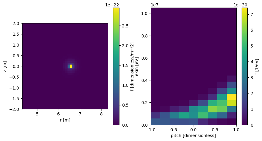
For thermal reactants, one can use toroidal coordinates \((\rho,\theta,\phi)\) as spatial grid, in which case the product distributions are also in toroidal coordinates. Using toroidal coordinates is especially useful for generating markers for stellarator simulations.
[6]:
a5.afsi.thermal(
    "DT_He4n", nmc=1000,
    rho=np.linspace(0, 1, 50),
    theta=np.linspace(0, 360, 10),
    )

alphadist = a5.data.active.getdist("prod1")
alphadist.integrate(time=np.s_[:], charge=np.s_[:], phi=np.s_[:])

rzdist  = alphadist.integrate(copy=True, ppar=np.s_[:], pperp=np.s_[:])
momdist = alphadist.integrate(copy=True, rho=np.s_[:], theta=np.s_[:])

fig = plt.figure(figsize=(10,5))
ax1 = fig.add_subplot(1,2,1)
ax2 = fig.add_subplot(1,2,2)

rzdist.plot(axes=ax1)
momdist.plot(axes=ax2)

plt.show()
AFSI5
Tag 6290a22
Branch docs

Note: Output file /home/runner/work/ascot5/ascot5/doc/tutorials/ascot.h5 is already present.

The qid of this run is 1975670910

Done
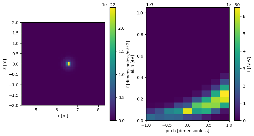
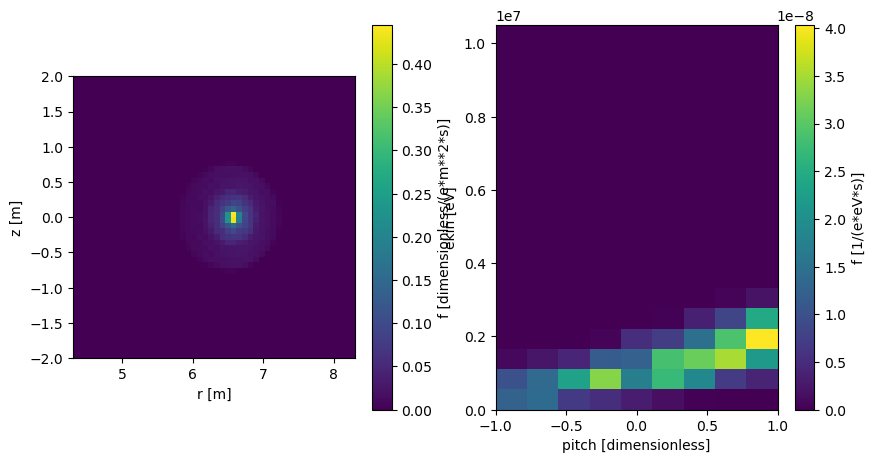
Next, we run the beam-thermal fusion between the deuterium beam (whose distribution was calculated earlier) and thermal deuterium. This time we use beamthermal function and provide the beam 5D function as an input. Note that this time we can’t specify a cylindrical grid for the outputs, as the same grid is used as in the beam distribution.
The results is again stored as a new run from which the data is read as usual. Take a note how the product distribution is strongly anisotropic; the product velocities consists of both the kinetic energy released in the reaction and the (beam) velocity that the reactants had.
[7]:
beamdist = a5.data.BEAMSD.getdist("5d")
a5.afsi.beamthermal("DD_Tp", beamdist, swap=True)

alphadist = a5.data.active.getdist("prod1", exi=True, ekin_edges=20, pitch_edges=10)
rzdist  = alphadist.integrate(copy=True, phi=np.s_[:], ekin=np.s_[:], pitch=np.s_[:])
exidist = alphadist.integrate(copy=True, phi=np.s_[:], r=np.s_[:], z=np.s_[:])

fig = plt.figure(figsize=(10,5))
ax1 = fig.add_subplot(1,2,1)
ax2 = fig.add_subplot(1,2,2)

rzdist.plot(axes=ax1)
exidist.plot(axes=ax2)

plt.show()
AFSI5
Tag 6290a22
Branch docs

Note: Output file /home/runner/work/ascot5/ascot5/doc/tutorials/ascot.h5 is already present.

The qid of this run is 1185431819

Done
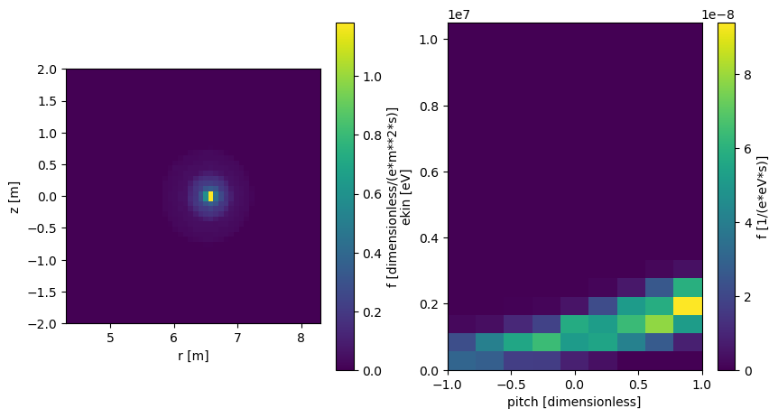
Finally, we demonstrate the beam-beam fusion. Providing the beambeam function with just a single distribution calculates the fusion product for the beam interacting with itself. The other beam would be provided with beam2 argument (which must have the same abscissae as the first beam distribution).
[8]:
a5 = Ascot("ascot.h5")
beamdist = a5.data.BEAMSD.getdist("5d")
a5.afsi.beambeam("DD_Tp", beamdist)

alphadist = a5.data.active.getdist("prod1", exi=True, ekin_edges=20, pitch_edges=10)
alphadist.integrate(time=np.s_[:], charge=np.s_[:]) # Distribution must be 5D

rzdist  = alphadist.integrate(copy=True, phi=np.s_[:], ekin=np.s_[:], pitch=np.s_[:])
exidist = alphadist.integrate(copy=True, phi=np.s_[:], r=np.s_[:], z=np.s_[:])

fig = plt.figure(figsize=(10,5))
ax1 = fig.add_subplot(1,2,1)
ax2 = fig.add_subplot(1,2,2)

rzdist.plot(axes=ax1)
exidist.plot(axes=ax2)

plt.show()
AFSI5
Tag 6290a22
Branch docs

Note: Output file /home/runner/work/ascot5/ascot5/doc/tutorials/ascot.h5 is already present.

The qid of this run is 0708434393

Done