Creating 3D field from coil geometry with BioSaw

This example shows how to run BioSaw to compute (error) field from coils.

BioSaw is a supporting tool that uses Biot-Savart law to compute 3D magnetic field input from a simple coil geometry represented by lines. It is used to calculate the toroidal field ripple due to finite number of TF coils or error fields produced by e.g. RMP coils.

To create a B_3DS input, we first need a file that contains B_2DS data:

import numpy as np
import unyt
import matplotlib.pyplot as plt
from a5py import Ascot

a5 = Ascot("ascot.h5", create=True)
a5.data.create_input("bfield analytical iter circular", splines=True, desc="AXISYMMETRIC")

'B_2DS_2502944457'

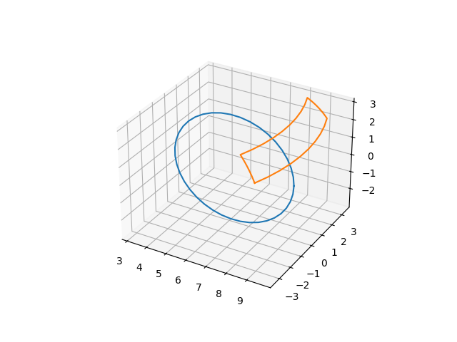
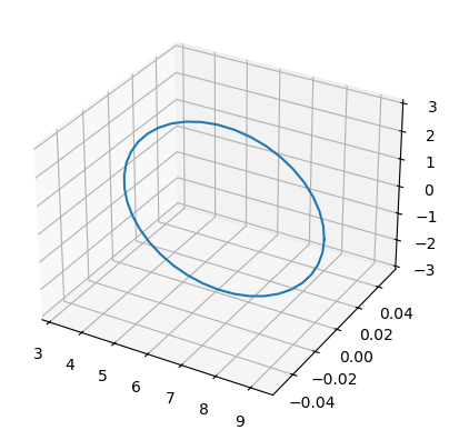
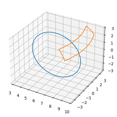
We now want to include the toroidal field ripple into this field. We begin by defining geometry for a single coil.

rad   = 3.0
ang   = np.linspace(0, 2*np.pi, 40)
coilx = rad * np.cos(ang) + 6.2
coily = np.zeros(ang.shape)
coilz = rad * np.sin(ang)
coilxyz = np.array([coilx, coily, coilz])

fig = plt.figure()
ax = fig.add_subplot(1,1,1, projection="3d")
ax.plot(coilx, coily, coilz)

plt.show()

Next we fix the number of TF field coils and set the coil current.

The number of TF coils is not given explicitly but it is dictated by the revolve argument. The field is calculated only once for a given coil, and then the field is rotated and added to get the total contribution from all TF coils. revolve defines the number of toroidal grid points (not the toroidal angle) the field is revolved in each rotation until we have gone whole turn. So if there are e.g. 18 TF coils, the number of grid points must be divisible by 18 and revolve is the number of grid points divided by the number of coils.

NOTE: If the coils or their positions do not possess a toroidal symmetry, define the coil geometry for each coil explicitly and set N=1.

The current can be given explicitly by current argument that sets the current in a single line segment. It can also be given indirectly, by setting what is the toroidal average of resulting \(B_\mathrm{phi}\) on the magnetic axis, and the current will be scaled accordingly.

The BioSaw is run via the Ascot object:

# Note that the Rz grid can be defined explicitly, but if it is not given then same
# is used as in the B_2DS data.
b3d = a5.biosaw.addto2d(
        coilxyz.T, phimin=0, phimax=360, nphi=180,
        revolve=10, b0=5.3)

a5.data.create_input("B_3DS", **b3d, desc="TFRIPPLE", activate=True)

'B_3DS_2159204756'

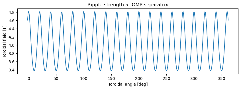
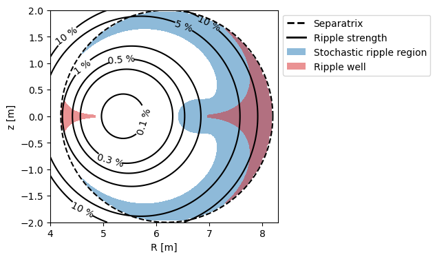
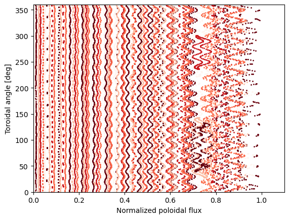
We can visualize the ripple to make sure everything looks right:

a5 = Ascot("ascot.h5")
rgrid = np.linspace(4.0,8.3,100) * unyt.m
zgrid = np.linspace(-2,2,100) * unyt.m
larmorrad = 0.01 # Use relevant larmor radius to plot the stochastic ripple region

fig = plt.figure(figsize=(10,3))
ax1 = fig.add_subplot(1,1,1)
ax1.set_title("Ripple strength at OMP separatrix")
fig = plt.figure(figsize=(6,4))
ax2 = fig.add_subplot(1,1,1)

a5.input_init(bfield=True)
a5.input_eval_ripple(rgrid, zgrid, larmorrad, plot=True, axes1=ax1, axes2=ax2)
a5.input_plotrhocontour(linestyle="--", color="black", axes=ax2)
a5.input_free()

# Add legend
from matplotlib.lines import Line2D
from matplotlib.patches import Patch
legend = [
    Line2D([0], [0], color="black", ls="--", lw=2, label="Separatrix"),
    Line2D([0], [0], color="black", lw=2, label="Ripple strength"),
    Patch(facecolor="C0", alpha=0.5, label="Stochastic ripple region"),
    Patch(facecolor="C3", alpha=0.5, label="Ripple well"),
]
ax2.legend(handles=legend, loc="upper left", bbox_to_anchor=(1,1))

plt.show()

The other case where BioSaw is used is to add a 3D peturbation to an already existing 3D field. This works in a similar way, except now the coil current must be set explicitly and we are not free to chose the cylindrical grid but has to use one that exists already.

def verticalpart(pol1, pol2, phi):
    rad   = 4.0
    ang   = np.linspace(pol1.to("rad"), pol2.to("rad"), 20)*unyt.deg
    r = rad * np.cos(ang) + 6.2
    coilx = r * np.cos(phi)
    coily = r * np.sin(phi)
    coilz = rad * np.sin(ang)
    return coilx, coily, coilz

def horizontalpart(phi1, phi2, pol):
    r = 6.2 + 4.0 * np.cos(pol)
    phi = np.linspace(phi1.to("rad"), phi2.to("rad"), 10)
    coilx = r * np.cos(phi)
    coily = r * np.sin(phi)
    coilz = 4.0 * np.sin(pol) * np.ones((10,))
    return coilx, coily, coilz

rmpx, rmpy, rmpz = verticalpart(30*unyt.deg, 50*unyt.deg, -20*unyt.deg)
x, y, z = horizontalpart(-20*unyt.deg, 20*unyt.deg, 50*unyt.deg)
rmpx = np.append(rmpx, x[1:])
rmpy = np.append(rmpy, y[1:])
rmpz = np.append(rmpz, z[1:])
x, y, z = verticalpart(50*unyt.deg, 30*unyt.deg, 20*unyt.deg)
rmpx = np.append(rmpx, x[1:])
rmpy = np.append(rmpy, y[1:])
rmpz = np.append(rmpz, z[1:])
x, y, z = horizontalpart(20*unyt.deg, -20*unyt.deg, 30*unyt.deg)
rmpx = np.append(rmpx, x[1:])
rmpy = np.append(rmpy, y[1:])
rmpz = np.append(rmpz, z[1:])

fig = plt.figure()
ax = fig.add_subplot(1,1,1, projection="3d")
rmpxyz = np.array([rmpx, rmpy, rmpz])
ax.plot(coilxyz[0,:], coilxyz[1,:], coilxyz[2,:])
ax.plot(rmpxyz[0,:], rmpxyz[1,:], rmpxyz[2,:])

plt.show()

b3d = a5.biosaw.addto3d(rmpxyz.T, revolve=90, current=30e4, b3d=a5.data.bfield.TFRIPPLE.read())

a5.data.create_input("B_3DS", **b3d, desc="RMP", activate=True)

'B_3DS_4047239463'

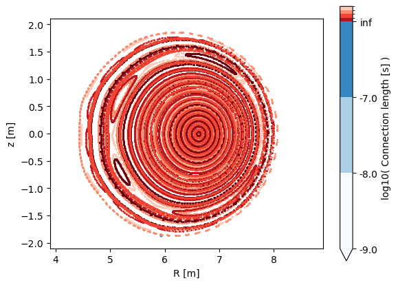
Visualize the results with Poincaré plots:

a5 = Ascot("ascot.h5")
a5.data.create_input("wall_2D")
a5.data.create_input("plasma_1D")
a5.data.create_input("E_TC")
a5.data.create_input("N0_3D")
a5.data.create_input("Boozer")
a5.data.create_input("MHD_STAT")
a5.data.create_input("asigma_loc")

a5.simulation_initinputs()
mrk = a5.data.create_input("marker poincare", dryrun=True)
a5.simulation_initmarkers(**mrk)
opt = a5.data.create_input("options poincare", maxrho=True, tor=[0], pol=[0], dryrun=True)
a5.simulation_initoptions(**opt)
vrun = a5.simulation_run(printsummary=False)
vrun.plotorbit_poincare("tor 1", connlen=True)
vrun.plotorbit_poincare("pol 1")
a5.simulation_free()

/home/runner/work/ascot5/ascot5/a5py/templates/__init__.py:64: AscotUnitWarning: Argument(s) tor, pol given without dimensions (assumed degree, degree)
  return template(**kwargs)

In the event that you wish to calculate the field due to coil(s) explicitly, without converting them to input, use a5.biosaw.calculate directly.