Simulating fast ion slowing-down process

This example shows how to run a fast-ion slowing-down simulation which is the bread-and-butter for ASCOT5.

We begin this example by generating some general input. For slowing-down simulations we need at least bfield and plasma inputs to contain real data:

import numpy as np
import unyt
import matplotlib.pyplot as plt
from a5py import Ascot

a5 = Ascot("ascot.h5", create=True)

# Use analytical field since it is fast to interpolate
a5.data.create_input("bfield analytical iter circular", desc="ANALYTICAL")

# DT-plasma
nrho   = 101
rho    = np.linspace(0, 2, nrho).T
edens  = 2e21 * np.ones((nrho, 1))
etemp  = 1e4  * np.ones((nrho, 1))
idens  = 1e21 * np.ones((nrho, 2))
itemp  = 1e4  * np.ones((nrho, 1))

edens[rho>1, :] = 1
idens[rho>1, :] = 1

pls = {
    "nrho" : nrho, "nion" : 2, "rho" : rho,
    "anum" : np.array([2, 3]), "znum" : np.array([1, 1]),
    "mass" : np.array([2.014, 3.016]), "charge" : np.array([1, 1]),
    "edensity" : edens, "etemperature" : etemp,
    "idensity" : idens, "itemperature" : itemp}
a5.data.create_input("plasma_1D", **pls, desc="FLATDT")

# These inputs are not relevant for this tutorial
a5.data.create_input("wall rectangular")
a5.data.create_input("E_TC")
a5.data.create_input("N0_1D")
a5.data.create_input("Boozer")
a5.data.create_input("MHD_STAT")
a5.data.create_input("asigma_loc")
print("Inputs created")

Inputs created

Next we create alpha source distribution using AFSI, but one could use BBNBI5 to generate beam ions or some other tool. This and the next step, where we sample markers from the alpha distribution, are covered in separate tutorials.

# Grid spanning the whole plasma
rmin =  4.2; rmax = 8.2; nr = 50
zmin = -2.0; zmax = 2.0; nz = 50

# Run AFSI which creates a fusion alpha distribution
a5.afsi.thermal(
    "DT_He4n", rmin, rmax, nr, zmin, zmax, nz,
    minphi=0, maxphi=2*np.pi, nphi=1, nmc=100,
    minppara=-1.3e-19, maxppara=1.3e-19, nppara=80,
    minpperp=0, maxpperp=1.3e-19, npperp=40)

# Convert to E-xi as then we can make dist more compact in momentum space
alphadist = a5.data.active.getdist("prod1", exi=True, ekin_edges=20, pitch_edges=10)
alphadist.integrate(time=np.s_[:], charge=np.s_[:]) # Distribution must be 5D


# Plot the distribution
#rzdist  = alphadist.integrate(copy=True, phi=np.s_[:], ppar=np.s_[:], pperp=np.s_[:])
rzdist  = alphadist.integrate(copy=True, phi=np.s_[:], ekin=np.s_[:], pitch=np.s_[:])
exidist = alphadist.integrate(copy=True, phi=np.s_[:], r=np.s_[:], z=np.s_[:])

fig = plt.figure()
ax1 = fig.add_subplot(1,2,1)
ax2 = fig.add_subplot(1,2,2)

rzdist.plot(axes=ax1)
exidist.plot(axes=ax2)

plt.show()

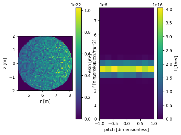
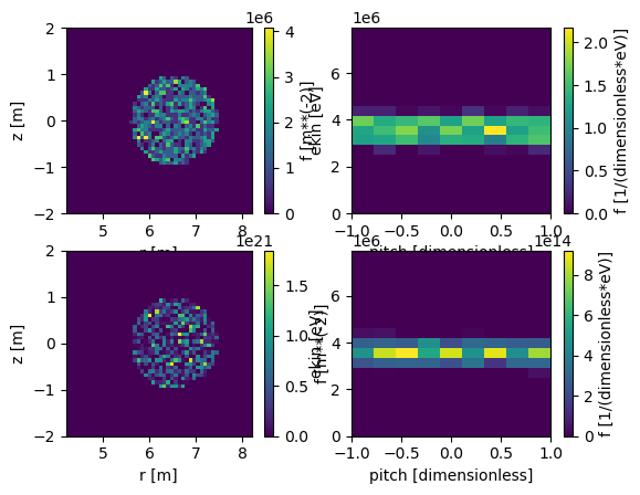
Markers are created from the fusion source distribution by first initializing marker distribution from a flat radial profile, and then assigning weights from the alpha birth distribution. In this tutorial we only initialize markers at the core to avoid losses.

# Create marker distribution. Here we just initialize markers evenly in rho for convenience
rho  = np.linspace(0, 0.5, 2)
prob = 0.5 * np.ones((2,))
a5.input_init(bfield=True)
markerdist = a5.markergen.rhoto5d(
    rho, prob, alphadist.abscissa_edges("r"),
    alphadist.abscissa_edges("phi"),  alphadist.abscissa_edges("z"),
    alphadist.abscissa_edges("ekin"), alphadist.abscissa_edges("pitch"))
a5.input_free()

# Create markers and take weights from the alpha distribution
mrk, mrkdist, prtdist = a5.markergen.generate(
    10**3, 4.002*unyt.amu, 2.0*unyt.e, 4, 2, alphadist, markerdist=markerdist,
    minweight=1e-10, return_dists=True)
a5.data.create_input("gc", **mrk, desc="ALPHAS")

# Plot the marker and particle distributions
rzmrk  = mrkdist.integrate(copy=True, phi=np.s_[:], ekin=np.s_[:], pitch=np.s_[:])
eximrk = mrkdist.integrate(copy=True, phi=np.s_[:], r=np.s_[:], z=np.s_[:])
rzprt  = prtdist.integrate(copy=True, phi=np.s_[:], ekin=np.s_[:], pitch=np.s_[:])
exiprt = prtdist.integrate(copy=True, phi=np.s_[:], r=np.s_[:], z=np.s_[:])

fig = plt.figure()
ax1 = fig.add_subplot(2,2,1)
ax2 = fig.add_subplot(2,2,2)
ax3 = fig.add_subplot(2,2,3)
ax4 = fig.add_subplot(2,2,4)

rzmrk.plot(axes=ax1)
eximrk.plot(axes=ax2)
rzprt.plot(axes=ax3)
exiprt.plot(axes=ax4)

plt.show()

AFSI5
Tag e389e6c
Branch docs

Note: Output file /home/runner/work/ascot5/ascot5/doc/tutorials/ascot.h5 is already present.

The qid of this run is 0245041939

Done

/home/runner/work/ascot5/ascot5/a5py/ascot5io/__init__.py:246: AscotUnitWarning: Argument(s) zeta given without dimensions (assumed rad)
  name = HDF5TOOBJ[inp].write_hdf5(

Now only options are missing. If the guiding-center approximation is valid, then using adaptive step is strongly recommended to accelerate the simulation. For other options, it is important to include energy limit as an end condition and activate orbit-following and Coulomb collisions in physics. Diagnostics can be whatever you like, though usually it makes little sense to collect orbit data. Here we collect 5D distribution which can be used to produce the slowing-down distribution.

from a5py.ascot5io.options import Opt

opt = Opt.get_default()
opt.update({
    # Simulation mode
    "SIM_MODE":2, "ENABLE_ADAPTIVE":1,
    # Setting max mileage above slowing-down time is a good safeguard to ensure
    # simulation finishes even with faulty inputs. Same with the CPU time limit.
    "ENDCOND_SIMTIMELIM":1, "ENDCOND_MAX_MILEAGE":0.5,
    "ENDCOND_CPUTIMELIM":1, "ENDCOND_MAX_CPUTIME":1.0e1,
    # The energy limit which separates a fast ion from thermal bulk is not well defined,
    # but we usually use Emin = 2 x Tion as the limit. Setting also a fixed minimum energy
    # is advised sine plasma temperature at the pedestal can be low.
    "ENDCOND_ENERGYLIM":1, "ENDCOND_MIN_ENERGY":2.0e3, "ENDCOND_MIN_THERMAL":2.0,
    # Physics
    "ENABLE_ORBIT_FOLLOWING":1, "ENABLE_COULOMB_COLLISIONS":1,
    # Distribution output
    "ENABLE_DIST_5D":1,
    "DIST_MIN_R":4.3,        "DIST_MAX_R":8.3,       "DIST_NBIN_R":50,
    "DIST_MIN_PHI":0,        "DIST_MAX_PHI":360,     "DIST_NBIN_PHI":1,
    "DIST_MIN_Z":-2.0,       "DIST_MAX_Z":2.0,       "DIST_NBIN_Z":50,
    "DIST_MIN_PPA":-1.3e-19, "DIST_MAX_PPA":1.3e-19, "DIST_NBIN_PPA":100,
    "DIST_MIN_PPE":0,        "DIST_MAX_PPE":1.3e-19, "DIST_NBIN_PPE":50,
    "DIST_MIN_TIME":0,       "DIST_MAX_TIME":1.0,    "DIST_NBIN_TIME":1,
    "DIST_MIN_CHARGE":1,     "DIST_MAX_CHARGE":3,    "DIST_NBIN_CHARGE":1,
})
a5.data.create_input("opt", **opt, desc="SLOWINGDOWN")

'opt_0754360888'

Now we are ready to simulate. Usually slowing-down simulations are expensive (especially with 3D magnetic field) but this one runs in a PC in a few minutes or so.

import subprocess
subprocess.run(["./../../build/ascot5_main", "--d=\"SDALPHA\""])
print("Simulation completed")

ASCOT5_MAIN
Tag e389e6c
Branch docs

Initialized MPI, rank 0, size 1.

Reading and initializing input.

Input file is ascot.h5.

Reading options input.
Active QID is 0754360888
Options read and initialized.

Reading magnetic field input.
Active QID is 4156884817

Analytical tokamak magnetic field (B_GS)
Psi at magnetic axis (6.618 m, -0.000 m)
-5.410 (evaluated)
-5.410 (given)
Magnetic field on axis:
B_R = 0.000 B_phi = 4.965 B_z = -0.000
Number of toroidal field coils 0
Estimated memory usage 0.0 MB
Magnetic field read and initialized.

Reading electric field input.
Active QID is 3103999104

Trivial Cartesian electric field (E_TC)
E_x = 0.000000e+00, E_y = 0.000000e+00, E_z = 0.000000e+00
Estimated memory usage 0.0 MB
Electric field read and initialized.

Reading plasma input.
Active QID is 2389566788

1D plasma profiles (P_1D)
Min rho = 0.00e+00, Max rho = 2.00e+00, Number of rho grid points = 101, Number of ion species = 2
Species Z/A  charge [e]/mass [amu] Density [m^-3] at Min/Max rho    Temperature [eV] at Min/Max rho
   1  /  2     1  /  2.014             1.00e+21/1.00e+00                1.00e+04/1.00e+04
   1  /  3     1  /  3.016             1.00e+21/1.00e+00                1.00e+04/1.00e+04
[electrons]   -1  /  0.001             2.00e+21/1.00e+00                1.00e+04/1.00e+04
Quasi-neutrality is (electron / ion charge density) 2.00
Estimated memory usage 0.0 MB
Plasma data read and initialized.

Reading neutral input.
Active QID is 1427632246

1D neutral density and temperature (N0_1D)
Grid:  nrho =    3   rhomin = 0.000   rhomax = 2.000
 Number of neutral species = 1
Species Z/A   (Maxwellian)
        1/  1 (1)
Estimated memory usage 0.0 MB
Neutral data read and initialized.

Reading wall input.
Active QID is 0427994176

2D wall model (wall_2D)
Number of wall elements = 20, R extend = [4.10, 8.40], z extend = [-3.90, 3.90]
Estimated memory usage 0.0 MB
Wall data read and initialized.

Reading boozer input.
Active QID is 0870302341

Boozer input
psi grid: n =    6 min = 0.000 max = 1.000
thetageo grid: n =   18
thetabzr grid: n =   10
Boozer data read and initialized.

Reading MHD input.
Active QID is 3002357965

MHD (stationary) input
Grid: nrho =    6 rhomin = 0.000 rhomax = 1.000

Modes:
(n,m) = ( 1, 3) Amplitude = 0.1 Frequency =   1 Phase =   0
(n,m) = ( 2, 4) Amplitude =   2 Frequency = 1.5 Phase = 0.785
Estimated memory usage 0.0 MB
MHD data read and initialized.

Reading atomic reaction input.
Active QID is 2951314059

Found data for 1 atomic reactions:
Reaction number / Total number of reactions = 1 / 1
  Reactant species Z_1 / A_1, Z_2 / A_2     = 1 / 1, 1 / 1
  Min/Max energy                            = 1.00e+03 / 1.00e+04
  Min/Max density                           = 1.00e+18 / 1.00e+20
  Min/Max temperature                       = 1.00e+03 / 1.00e+04
  Number of energy grid points              = 3
  Number of density grid points             = 4
  Number of temperature grid points         = 5
Estimated memory usage 0.0 MB
Atomic reaction data read and initialized.

Reading marker input.
Active QID is 2164791589

Loaded 1000 guiding centers.
Marker data read and initialized.

All input read and initialized.

Initializing marker states.
Estimated memory usage 0.0 MB.
Marker states initialized.
Initialized diagnostics, 95.4 MB.

Preparing output.
Note: Output file ascot.h5 is already present.

The qid of this run is 0489927881

Inistate written.
Simulation begins; 4 threads.
Simulation complete.
Simulation finished in 55.084642 s
Endstate written.

Combining and writing diagnostics.

Writing diagnostics output.

Writing 5D distribution.

Diagnostics output written.
Diagnostics written.

Summary of results:
     1000 markers had end condition Thermalization

          No markers were aborted.

Done.
Simulation completed

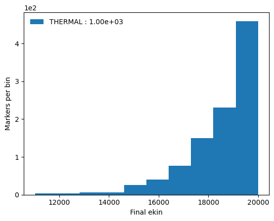
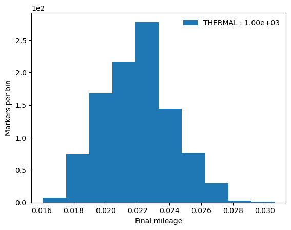
Now the first thing to check in the results is that the markers actually slowed-down. Therefore we look at the end conditions, final energy, and mileage which gives us the slowing-down time.

a5 = Ascot("ascot.h5") # Re-read the data
print(a5.data.active.getstate_markersummary())
a5.data.active.plotstate_histogram("end ekin")
a5.data.active.plotstate_histogram("end mileage")

([(np.int64(1000), 'THERMAL')], [])

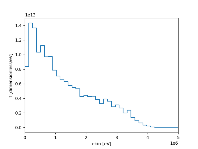
Looks reasonable! Now let us look at the slowing-down distribution.

d = a5.data.active.getdist("5d", exi=True, ekin_edges=np.linspace(0,5e6,40), pitch_edges=2)
d.integrate(time=np.s_[:], charge=np.s_[:], phi=np.s_[:], r=np.s_[:], z=np.s_[:], pitch=np.s_[:])
d.plot()

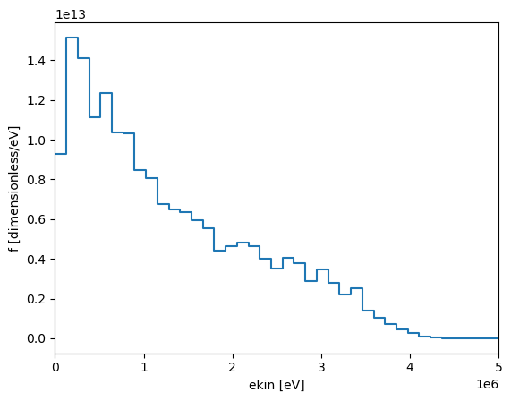
One can note that there might be markers above the initial energy, i.e. some markers have actually gained energy! However, this “up-scattering” is fine because the collision operator contains a stochastic component and the main thing is that the whole population cools on average. And, as we checked earlier, there were no energetic markers left at the end of the simulation so all markers either slowed-down or were lost.

Finally, it is a good idea to check the energy-pitch distribution as well.

d = a5.data.active.getdist("5d", exi=True, ekin_edges=20, pitch_edges=10)
d.integrate(time=np.s_[:], charge=np.s_[:], phi=np.s_[:], r=np.s_[:], z=np.s_[:])
d.plot()

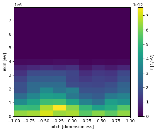
Here we want to verify that marker pitch has not accumulated in some point because the physics governs that the pitch scattering should make the pitch distribution close to even in the end. Initially there is little pitch scattering, since fast particles are usually born above the critical energy,

\[v_\mathrm{crit} = v_\mathrm{th} \left(\frac{3 \sqrt{\pi}}{4}\frac{m_e}{m_\mathrm{ion}}\right)^{1/3}.\]

Above the critical energy we should see little pitch scattering as the fast ions mostly collide with electrons, but this changes below the critical energy as now the ion-ion collision frequency is higher than the electron-ion collision frequency.

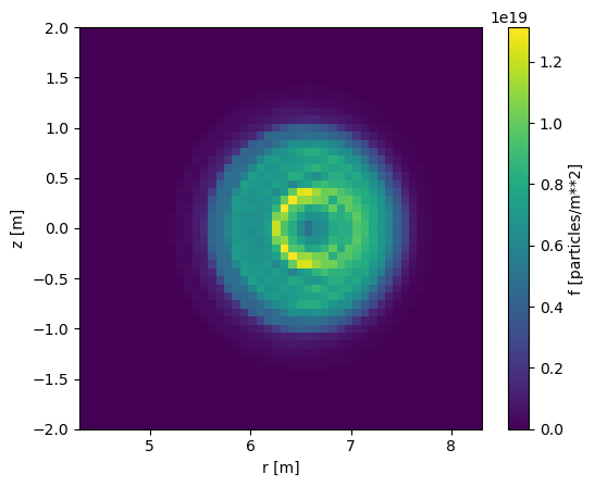
This concludes the tutorial. Here’s a complementary fast-ion slowing-down density to brighten your day:

d = a5.data.active.getdist("5d")
d.integrate(time=np.s_[:], charge=np.s_[:], phi=np.s_[:], ppar=np.s_[:], pperp=np.s_[:])
d.plot()