Generating Poincaré plots

This example shows how to generate Poincaré plots, a.k.a. puncture plots, with ASCOT5. These plots are generated by tracing markers and recording their position each time a marker crosses a poloidal or toroidal plane. They are mainly used to visualize magnetic field structures and particle resonances. Poincaré plots can be made for both field lines and physical particles.

First we create a simple test case (skip this part when doing actual studies).

import numpy as np
from a5py import Ascot

a5 = Ascot("ascot.h5", create=True)
a5.data.create_input("options tutorial")
a5.data.create_input("bfield analytical iter circular")
a5.data.create_input("wall rectangular")
a5.data.create_input("plasma flat")
a5.data.create_input("E_TC", exyz=np.array([0,0,0]))
a5.data.create_input("N0_3D")
a5.data.create_input("Boozer")
a5.data.create_input("MHD_STAT")
a5.data.create_input("asigma_loc")
print("Inputs created")

Inputs created

Next we create markers and options for the Poincaré simulation. There is nothing extraordinary in these inputs: the markers are just initialized at uniform interals in radius and the options disable all other physics except orbit-following, set proper end conditions, and enable Poincaré data collection.

Generating markers involves mapping (rho,theta) coordinates to (R,z) which is why magnetic field initialization is required.

a5.input_init(bfield=True)
a5.data.create_input("marker poincare", activate=True, desc="PNCR Poincare")
a5.input_free()
print(a5.data.marker.active.get_desc())

PNCR Poincare

a5.data.create_input("options poincare", maxrho=True, activate=True, desc="PNCR Poincare")
print(a5.data.options.active.get_desc())

PNCR Poincare

Now you can either run the simulation using ascot5_main or, as we do here, utilize the live simulation support.

a5.simulation_initinputs()
mrk = a5.data.marker.active.read()
a5.simulation_initmarkers(**mrk)
opt = a5.data.options.active.read()
a5.simulation_initoptions(**opt)
vrun = a5.simulation_run(printsummary=True)
print("Done")

/home/runner/work/ascot5/ascot5/a5py/ascotpy/libsimulate.py:327: AscotUnitWarning: Argument(s) r, phi, z, time given without dimensions (assumed m, degree, m, s)
  r, phi, z, t, pitch, w, ids = parse(

Done

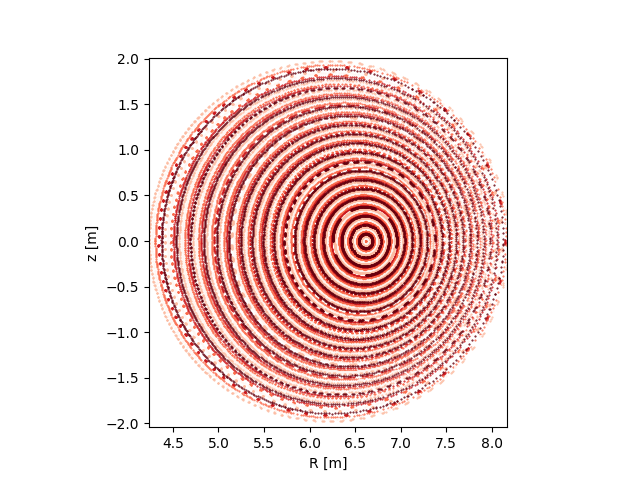
Now we can plot the results.

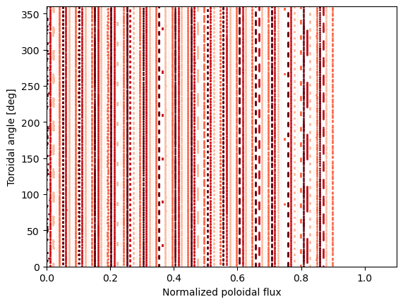
vrun.plotorbit_poincare("pol 1")

Remember to free resources if you ran a live simulation.

a5.simulation_free()

Summary of results:
       99 markers had end condition Max toroidal orbits
        1 markers had end condition Max rho

          No markers were aborted.

That was the basic method of creating Poincaré plots. It is strongly advised to generate a Poincaré plot when using a new magnetic field data for the first time to verify the field quality. Note that if the field quality is abysmal, the adaptive time-stepping used in field-line tracing might get stuck, which can be somewhat mitigated by tracing electron guiding centers with a fixed time step instead or setting the maximum CPU time limit end condition active. Furthermore, the Poincaré marker generation might fail if rho becomes imaginary near the axis due to incorrect normalization, so always check that with the input_plotrz method.

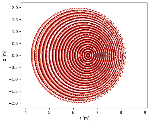
Poincaré plots made with physical particles can be created in a following way, i.e. by providing species name, energy and pitch. Poincaré plots for poloidally trapped particles is not yet fully supported.

a5.input_init(bfield=True)
a5.data.create_input("marker poincare", species="alpha", energy=3.5e6, pitch=0.9, activate=True,
                     desc="PRTPNCR Particle poincare")
a5.input_free()
print(a5.data.marker.active.get_desc())

PRTPNCR Particle poincare

This change alone doesn’t affect anything unless we change the simulation mode from field-line to guiding-center. Gyro-orbit simulations are also supported.

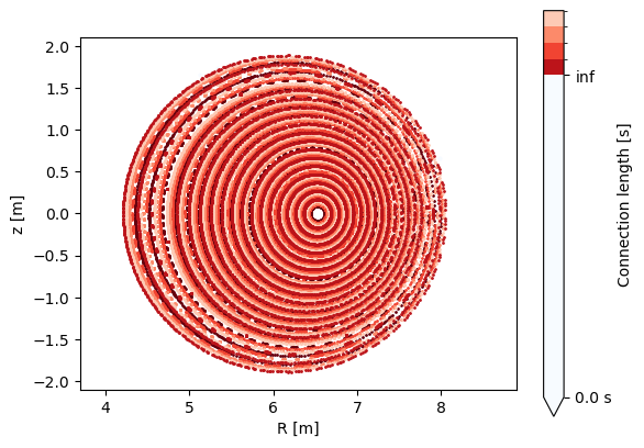
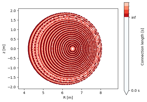
Making multiple Poincaré plots at different planes simultaneously is also supported as we demonstrate here.

a5.data.create_input("options poincare", maxrho=True, simmode=2, tor=[0, 180], pol=[0, 180], activate=True,
                     desc="PRTPNCR Particle poincare")
print(a5.data.options.active.get_desc())

PRTPNCR Particle poincare

/home/runner/work/ascot5/ascot5/a5py/templates/__init__.py:64: AscotUnitWarning: Argument(s) tor, pol given without dimensions (assumed degree, degree)
  return template(**kwargs)

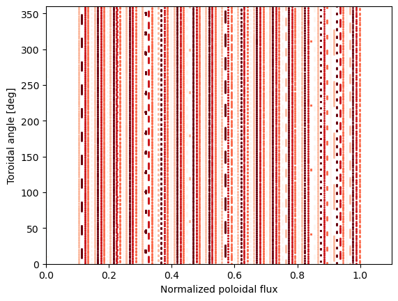
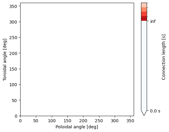
Note that we set maxrho=True, which dictates that markers are only traced until they exit the separatrix. The default behaviour is to trace markers all the way to the wall (however, this is cannot be done in this test input case where the mock-up wall is in a galaxy far far away). By tracing markers all the way to the wall, the connection length in the plots is the proper connection length, i.e. the distance along the orbit to the wall.

Now is the time to run the simulation.

a5.simulation_initinputs()
mrk = a5.data.marker.active.read()
a5.simulation_initmarkers(**mrk)
opt = a5.data.options.active.read()
a5.simulation_initoptions(**opt)
vrun = a5.simulation_run(printsummary=True)
print("Done")

/home/runner/work/ascot5/ascot5/a5py/ascotpy/libsimulate.py:297: AscotUnitWarning: Argument(s) r, phi, z, time, mass, charge, energy, zeta given without dimensions (assumed m, degree, m, s, amu, e, eV, rad)
  r, phi, z, t, m, q, energy, pitch, zeta, anum, znum, w, ids = parse(

Done

Plot all Poincarés.

vrun.plotorbit_poincare("pol 1")
vrun.plotorbit_poincare("pol 2")
vrun.plotorbit_poincare("tor 1")
vrun.plotorbit_poincare("tor 2")
vrun.plotorbit_poincare("rad 1")

(Free the resources.)

a5.simulation_free()

Summary of results:
       90 markers had end condition Max toroidal orbits
       10 markers had end condition Max rho

          No markers were aborted.

Done.