Modelling neutral beam injection with BBNBI
This example shows how to generate beam ions with BBNBI5.
In order to run BBNBI, you’ll need to compile it separately with make bbnbi5 and the resulting binary will be in the build folder. Once that is done, we initialize some test data. BBNBI requires magnetic field, plasma, neutral, wall, and atomic data to be present.
NOTE: Currently atomic data is not used even though it is required; it is a placeholder for future development.
Here we use spline interpolated magnetic field and 3D wall to demonstrate specific aspects of BBNBI.
[1]:
import numpy as np
import unyt
import matplotlib.pyplot as plt
from a5py import Ascot

a5 = Ascot("ascot.h5", create=True)

# Use splines for a more realistic case
a5.data.create_input("bfield analytical iter circular", splines=True,
                     desc="SPLINE2D")

nrho  = 101
rho   = np.linspace(0, 2, nrho).T
prof  = (rho<=1)*(1.0 - rho**(3.0/2))**3 + 1e-6
vtor  = np.zeros((nrho, 1))
edens = 2e20 * prof
etemp = 1e4  * np.ones((nrho, 1))
idens = 1e20 * np.reshape(prof,(nrho,1))
itemp = 1e4  * np.ones((nrho, 1))

edens[rho>=1] = 1
idens[rho>=1] = 1

pls = {
    "nrho" : nrho, "nion" : 1, "rho" : rho, "vtor": vtor,
    "anum" : np.array([2]), "znum" : np.array([1]),
    "mass" : np.array([2.014]), "charge" : np.array([1]),
    "edensity" : edens, "etemperature" : etemp,
    "idensity" : idens, "itemperature" : itemp}
a5.data.create_input("plasma_1D", **pls, desc="FLATDT")

from a5py.ascot5io.wall import wall_3D
rad  = 2.1
pol  = np.linspace(0, 2*np.pi, 180)
wall = {"nelements":180,
        "r":6.2 + rad*np.cos(pol), "z":0.0 + rad*np.sin(pol)}
wall = wall_3D.convert_wall_2D(180, **wall)
a5.data.create_input("wall_3D", **wall, desc="ROTATED")

a5.data.create_input("N0_1D")
a5.data.create_input("asigma_loc")

print("Inputs created")
/home/runner/work/ascot5/ascot5/a5py/routines/plotting.py:35: UserWarning: Could not import cKDTree and alphashape. 3D surface plotting disabled.
  warnings.warn(
Inputs created
One input that is entirely BBNBI specific is the NBI input that contains a bundle of injectors. The injector data defines the geometry of the injectory, the injected species, its energy (distribution), and power. Often one does not need to specify the geometry as the data already exists.
NOTE: Injector specifications exists for the following machines: ITER, JET, ASDEX Upgrade, MAST-U, JT-60SA, NSTX, and TCV. These cannot be shared publicly within the ASCOT5 repository, so please contact the maintainers to gain access to the data.
For this tutorial, we use the method a5py.ascot5io.nbi.NBI.generate which creates a simplified injector.
[2]:
from a5py.ascot5io.nbi  import NBI
inj = NBI.generate(r=10.0, phi=10.0, z=0.0, tanrad=-6.0, focallen=1.0,
                   dgrid=[0.23, 0.52], nbeamlet=1, anum=2, znum=1,
                   mass=2.0141, energy=1e6, efrac=[1.0, 0.0, 0.0],
                   power=1e6, tilt=0.1,
                   div=[np.deg2rad(0.95)/2, np.deg2rad(0.95)/2])
a5.data.create_input("nbi", **{"ninj":1, "injectors":[inj]},
                     desc="INJECTORS")
[2]:
'nbi_1596760898'
BBNBI shares some of the options with the main program. Mainly the distribution output settings (which are optional).
[3]:
from a5py.ascot5io.options import Opt

opt = Opt.get_default()
opt.update({
    "ENABLE_DIST_5D":1,
    "DIST_MIN_R":4.3,        "DIST_MAX_R":8.3,       "DIST_NBIN_R":50,
    "DIST_MIN_PHI":0,        "DIST_MAX_PHI":360,     "DIST_NBIN_PHI":1,
    "DIST_MIN_Z":-2.0,       "DIST_MAX_Z":2.0,       "DIST_NBIN_Z":50,
    "DIST_MIN_PPA":-1.3e-19, "DIST_MAX_PPA":1.3e-19, "DIST_NBIN_PPA":100,
    "DIST_MIN_PPE":0,        "DIST_MAX_PPE":1.3e-19, "DIST_NBIN_PPE":50,
    "DIST_MIN_TIME":0,       "DIST_MAX_TIME":1.0,    "DIST_NBIN_TIME":1,
    # Note: The charge lower bound is inclusive, upper bound is not
    "DIST_MIN_CHARGE":1,     "DIST_MAX_CHARGE":2,    "DIST_NBIN_CHARGE":1,
})
a5.data.create_input("opt", **opt, desc="BEAMDEPOSITION")
[3]:
'opt_0389252115'
To run a simulation, BBNBI works in a similar fashion as ascot5_main. One notable difference is that BBNBI is not MPI parallelized. The total number of markers to be injected from all injectors is given as a command line parameter.
[4]:
import subprocess
subprocess.run(["./../../build/bbnbi5", "--n=10000", "--d=\"BEAMS\""])
print("Simulation completed")
BBNBI5
Tag 6290a22
Branch docs


Reading and initializing input.

Input file is ascot.h5.

Reading options input.
Active QID is 0389252115
Options read and initialized.

Reading magnetic field input.
Active QID is 3827447145

2D magnetic field (B_2DS)
Grid: nR =  120 Rmin = 4.000 Rmax = 8.500
      nz =  200 zmin = -4.000 zmax = 4.000
Psi at magnetic axis (6.618 m, -0.000 m)
-5.410 (evaluated)
-5.410 (given)
Magnetic field on axis:
B_R = 0.000 B_phi = 4.965 B_z = -0.000
Magnetic field read and initialized.

Reading plasma input.
Active QID is 0461566902

1D plasma profiles (P_1D)
Min rho = 0.00e+00, Max rho = 2.00e+00, Number of rho grid points = 101, Number of ion species = 1
Species Z/A  charge [e]/mass [amu] Density [m^-3] at Min/Max rho    Temperature [eV] at Min/Max rho
   1  /  2     1  /  2.014             1.00e+20/1.00e+00                1.00e+04/1.00e+04
[electrons]   -1  /  0.001             2.00e+20/1.00e+00                1.00e+04/1.00e+04
Toroidal rotation [rad/s] at Min/Max rho: 0.00e+00/0.00e+00
Quasi-neutrality is (electron / ion charge density) 1.50
Toroidal rotation [rad/s] at Min/Max rho: 0.00e+00/0.00e+00
Plasma data read and initialized.

Reading neutral input.
Active QID is 0936136085

1D neutral density and temperature (N0_1D)
Grid:  nrho =    3   rhomin = 0.000   rhomax = 2.000
 Number of neutral species = 1
Species Z/A   (Maxwellian)
        1/  1 (1)
Neutral data read and initialized.

Reading wall input.
Active QID is 3677743053

3D wall model (wall_3D)
Number of wall elements 64800
Spanning xmin = -8.400 m, xmax = 8.400 m
         ymin = -8.400 m, ymax = 8.400 m
         zmin = -2.200 m, zmax = 2.200 m
Wall data read and initialized.

Reading atomic reaction input.
Active QID is 2458329973

Found data for 1 atomic reactions:
Reaction number / Total number of reactions = 1 / 1
  Reactant species Z_1 / A_1, Z_2 / A_2     = 0 / 0, 0 / 0
  Min/Max energy                            = 1.00e+03 / 1.00e+04
  Min/Max density                           = 1.00e+18 / 1.00e+20
  Min/Max temperature                       = 1.00e+03 / 1.00e+04
  Number of energy grid points              = 3
  Number of density grid points             = 4
  Number of temperature grid points         = 5
Atomic reaction data read and initialized.

Reading NBI input.
Active QID is 1596760898

NBI input
Number of injectors 1:

  Injector ID 1 (1 beamlets) Power: 1.0e+06
    Anum 2 Znum 1 mass 2.0e+00 amu energy 1.0e+06 eV
    Energy fractions: 1.0e+00 (Full) 0.0e+00 (1/2) 0.0e+00 (1/3)
NBI data read and initialized.

All input read and initialized.

Preparing output.
Note: Output file ascot.h5 is already present.

The qid of this run is 1576923371
Generated 10000 markers for injector 1.

Marker state written.

Writing diagnostics output.

Writing 5D distribution.

Diagnostics output written.

Done
Simulation completed
The results are stored as a (BBNBI) run group that can be accessed via Ascot object. Data and methods related to marker state, wall loads, and distributions are accessible. Note that this run does not have a separate ini and endstate but just a single state that corresponds to the marker final position.
[5]:
from a5py import Ascot
a5 = Ascot("ascot.h5")
r, z = a5.data.active.getstate("r", "z", mode="prt")

fig, ax = plt.subplots()
ax.scatter(r, z)
plt.show()
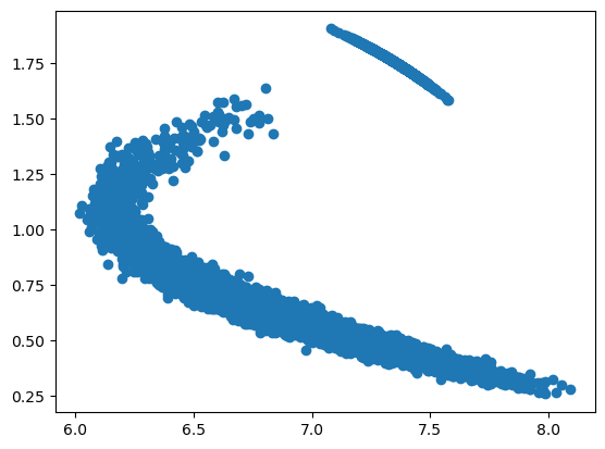
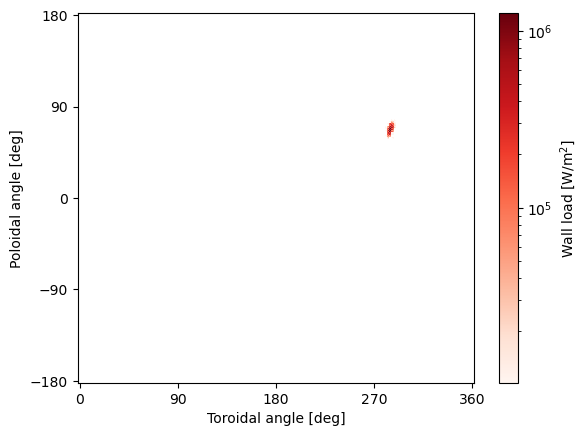
The plot above shows that some of the markers were not ionized but instead continued until they hit the wall on the opposite end, i.e., they became shinethrough. We can visualize the shinethrough with the same methods as are used to plot the wall loads.
[6]:
a5.input_init(bfield=True)
a5.data.active.plotwall_torpol()
a5.input_free()
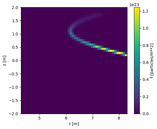
If distributions were collected, we can plot the beam deposition. Keep in mind that this is not a steady-state distribution but instead it shows the birth rate of beam ions.
[7]:
dist = a5.data.active.getdist("5d")
dist.integrate(phi=np.s_[:], ppar=np.s_[:], pperp=np.s_[:], charge=np.s_[:], time=np.s_[:])
dist.plot()
One can use either the above distribution to generate markers for the slowing down simulation (using the MarkerGenerator class) or use the ionized markers directly:
[8]:
ids = a5.data.active.getstate("ids", endcond="IONIZED")
mrk = a5.data.active.getstate_markers("gc", ids=ids)
print(mrk["n"])
print(mrk["charge"])
9995
[1. 1. 1. ... 1. 1. 1.] e