Tracing markers backwards in time

This example shows how to trace markers backwards in time.
For starters it is worth emphasizing that this tutorial is only for tracing marker orbits backwards in time and not for reverting the physical process. Activating the time reversal option, REVERSE_TIME=1, makes the time run backwards in simulations so that one can e.g. see the orbit at which a marker hit the wall or FILD. However, it does not reverse collisional or other stochastic process so these must be disabled. Use BMC for proper backwards Monte Carlo modelling that include these
processess and can properly run a slowing-down simulation in reverse.
First set up the test data.
[1]:
import numpy as np
import matplotlib.pyplot as plt
from a5py import Ascot

a5 = Ascot("ascot.h5", create=True)
a5.data.create_input("bfield analytical iter circular")
a5.data.create_input("plasma flat")
a5.data.create_input("E_TC")
a5.data.create_input("N0_1D")
a5.data.create_input("Boozer")
a5.data.create_input("MHD_STAT")
a5.data.create_input("asigma_loc")

print("Inputs created")
/home/runner/work/ascot5/ascot5/a5py/routines/plotting.py:35: UserWarning: Could not import cKDTree and alphashape. 3D surface plotting disabled.
  warnings.warn(
Inputs created
As for the wall, any wall data would do but we wish to do some nice visualizations in 3D so we choose a 3D wall for this exercise.
[2]:
from a5py.ascot5io.wall import wall_3D

rad  = 2.0
pol  = np.linspace(0, 2*np.pi, 181)[:-1]
w2d = {"nelements":180,
       "r":6.4 + rad*np.cos(pol), "z":rad*np.sin(pol)}
w3d = wall_3D.convert_wall_2D(180, **w2d)
a5.data.create_input("wall_3D", **w3d, desc="REVOLVED")
[2]:
'wall_3D_0264267289'
Now let’s create a few markers which we trace for a few moments as if we were modelling the slowing-down process. This is an ordinary forward in time simulation, we will use the results to run the reversed simulation (although there is nothing preventing from running the reversed simulation without the forward simulation).
[3]:
from a5py.ascot5io.marker import Marker
nmrk = 10
mrk = Marker.generate("gc", n=nmrk, species="alpha")
mrk["energy"][:] = 3.5e6
mrk["pitch"][:]  = 0.6
mrk["r"][:]      = np.linspace(7.6,8.0,nmrk)
a5.data.create_input("gc", **mrk, activate=True)

from a5py.ascot5io.options import Opt

opt = Opt.get_default()
opt.update({
    # Reversed time does not work well with the adaptive step at the moment so disable it
    "SIM_MODE":2, "ENABLE_ADAPTIVE":0,
    "ENDCOND_SIMTIMELIM":1, "ENDCOND_LIM_SIMTIME":1.0e-4, "ENDCOND_WALLHIT":1,
    "ENABLE_ORBIT_FOLLOWING":1, "ENABLE_COULOMB_COLLISIONS":1,
    "ENABLE_ORBITWRITE":1, "ORBITWRITE_MODE":1, "ORBITWRITE_INTERVAL":0,
    "ORBITWRITE_NPOINT":10**4,
})
a5.data.create_input("opt", **opt, desc="TIMEFORWARD", activate=True)
[3]:
'opt_3766525038'
Run the simulation
[4]:
import subprocess
subprocess.run(["./../../build/ascot5_main", "--d=\"GREATESTHITSVOL2\""])
print("Simulation completed")
ASCOT5_MAIN
Tag 6290a22
Branch docs

Initialized MPI, rank 0, size 1.

Reading and initializing input.

Input file is ascot.h5.

Reading options input.
Active QID is 3766525038
Options read and initialized.

Reading magnetic field input.
Active QID is 1326692302

Analytical tokamak magnetic field (B_GS)
Psi at magnetic axis (6.618 m, -0.000 m)
-5.410 (evaluated)
-5.410 (given)
Magnetic field on axis:
B_R = 0.000 B_phi = 4.965 B_z = -0.000
Number of toroidal field coils 0
Magnetic field read and initialized.

Reading electric field input.
Active QID is 1752787841

Trivial Cartesian electric field (E_TC)
E_x = 0.000000e+00, E_y = 0.000000e+00, E_z = 0.000000e+00
Electric field read and initialized.

Reading plasma input.
Active QID is 4074334807

1D plasma profiles (P_1D)
Min rho = 0.00e+00, Max rho = 1.00e+01, Number of rho grid points = 100, Number of ion species = 1
Species Z/A  charge [e]/mass [amu] Density [m^-3] at Min/Max rho    Temperature [eV] at Min/Max rho
   1  /  1     1  /  1.000             1.00e+21/1.00e+00                1.00e+04/1.00e+04
[electrons]   -1  /  0.001             1.00e+21/1.00e+00                1.00e+04/1.00e+04
Toroidal rotation [rad/s] at Min/Max rho: 0.00e+00/0.00e+00
Quasi-neutrality is (electron / ion charge density) 1.00
Toroidal rotation [rad/s] at Min/Max rho: 0.00e+00/0.00e+00
Plasma data read and initialized.

Reading neutral input.
Active QID is 3383709403

1D neutral density and temperature (N0_1D)
Grid:  nrho =    3   rhomin = 0.000   rhomax = 2.000
 Number of neutral species = 1
Species Z/A   (Maxwellian)
        1/  1 (1)
Neutral data read and initialized.

Reading wall input.
Active QID is 0264267289

3D wall model (wall_3D)
Number of wall elements 64800
Spanning xmin = -8.500 m, xmax = 8.500 m
         ymin = -8.500 m, ymax = 8.500 m
         zmin = -2.100 m, zmax = 2.100 m
Wall data read and initialized.

Reading boozer input.
Active QID is 0894340442

Boozer input
psi grid: n =    6 min = 0.000 max = 1.000
thetageo grid: n =   18
thetabzr grid: n =   10
Boozer data read and initialized.

Reading MHD input.
Active QID is 3161137393

MHD (stationary) input
Grid: nrho =    6 rhomin = 0.000 rhomax = 1.000

Modes:
(n,m) = ( 1, 3) Amplitude = 0.1 Frequency =   1 Phase =   0
(n,m) = ( 2, 4) Amplitude =   2 Frequency = 1.5 Phase = 0.785
MHD data read and initialized.

Reading atomic reaction input.
Active QID is 2618745550

Found data for 1 atomic reactions:
Reaction number / Total number of reactions = 1 / 1
  Reactant species Z_1 / A_1, Z_2 / A_2     = 0 / 0, 0 / 0
  Min/Max energy                            = 1.00e+03 / 1.00e+04
  Min/Max density                           = 1.00e+18 / 1.00e+20
  Min/Max temperature                       = 1.00e+03 / 1.00e+04
  Number of energy grid points              = 3
  Number of density grid points             = 4
  Number of temperature grid points         = 5
Atomic reaction data read and initialized.

Reading marker input.
Active QID is 2143041502

Loaded 10 guiding centers.
Marker data read and initialized.

All input read and initialized.

Initializing marker states.
Estimated memory usage 0.0 MB.
Marker states initialized.

Preparing output.
Note: Output file ascot.h5 is already present.

The qid of this run is 0547347207

Inistate written.
Simulation begins; 4 threads.
Simulation complete.
Simulation finished in 0.694489 s
Endstate written.

Combining and writing diagnostics.

Writing diagnostics output.
Writing orbit diagnostics.

Diagnostics output written.
Diagnostics written.

Summary of results:
        7 markers had end condition Sim time limit
        3 markers had end condition Wall collision

          No markers were aborted.

Done.
Simulation completed
Few markers hit the wall. We select one of them and run the orbit backwards in time.
[5]:
a5 = Ascot("ascot.h5")

# Pick one of the markers that hit the wall
ids = a5.data.active.getstate("ids", endcond="wall")[0]

# When converting endstate to marker input, the input type and the simulation
# mode that was used should preferably match
mrk = a5.data.active.getstate_markers("gc", ids=ids)

opt = a5.data.active.options.read()
opt.update({
    # Reverse time and turn off the collisions
    "REVERSE_TIME":1, "ENABLE_COULOMB_COLLISIONS":0,
    # When using the reversed time, the simulation is stopped if time < LIM_SIMTIME.
    # To follow marker back to its original position, we set LIM_SIMTIME=0 which was
    # the marker time at the start of the forward simulation.
    # Note that MAX_MILEAGE works same way both in forward and reversed simulations.
    "ENDCOND_LIM_SIMTIME":0.0,
    "ENDCOND_WALLHIT":0
})
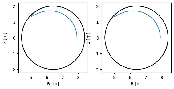
Since we are only tracing a single marker, and we are only interested in its orbit, the reversed simulation can be done conveniently using the virtual run (but ordinary run would work as well).
Run the simulation and plot both the forward orbit and the reversed orbit.
[6]:
a5.simulation_initinputs()
a5.simulation_initmarkers(**mrk)
a5.simulation_initoptions(**opt)
vrun = a5.simulation_run(printsummary=False)

fig = plt.figure()
ax1 = fig.add_subplot(1,2,1)
ax2 = fig.add_subplot(1,2,2)

a5.data.active.plotorbit_trajectory("r", "z", ids=mrk["ids"], axes=ax1)
a5.input_plotwallcontour(axes=ax1)

vrun.plotorbit_trajectory("r", "z", axes=ax2)
a5.input_plotwallcontour(axes=ax2)

plt.show()

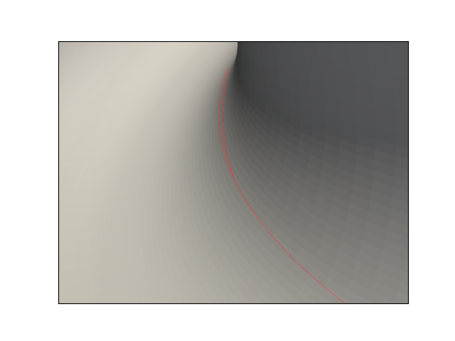
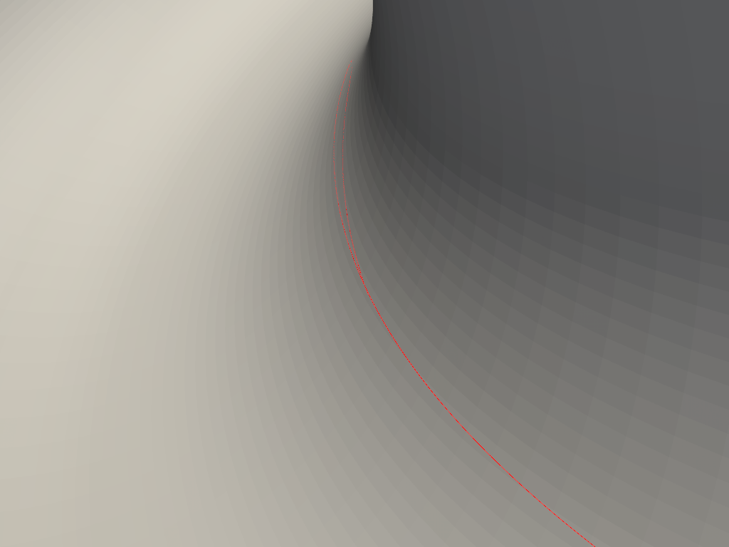
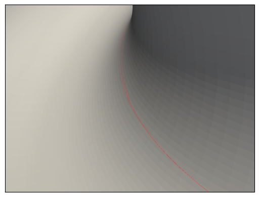
This is how time reversed simulations are done. They can be used to map the phase-space region where losses originate (for collisionless losses) or to make nice visualizations of marker orbits when they hit the wall or FILD.
[7]:
fig, ax = plt.subplots()
vrun.plotwall_3dstill(cpos=(-7.0,0.0,0.5), cfoc=(-3.8,-3.5,1.5), cang=(0,-20,-90), orbit=mrk["ids"], axes=ax)
a5.simulation_free()
/home/runner/work/ascot5/ascot5/a5py/routines/plotting.py:1277: UserWarning: Failed to use notebook backend:

No module named 'trame'

Falling back to a static output.
  p.show()

