Simulating test particle response to MHD

It is possible to include rotating helical perturbations to simulations to e.g. study fast ion response to Alfvén eigenmodes and this tutorial shows how to do it.

We begin by generating a test case consisting of a 2D tokamak.

import numpy as np
import unyt
import matplotlib.pyplot as plt
from a5py import Ascot

a5 = Ascot("ascot.h5", create=True)

# The magnetic input has to be B_2DS format so we use splines=True to convert
# the analytical field to splines
a5.data.create_input("bfield analytical iter circular", splines=True)
a5.data.create_input("wall_2D")
a5.data.create_input("plasma_1D")
a5.data.create_input("E_TC")
a5.data.create_input("N0_1D")
a5.data.create_input("asigma_loc")

print("Inputs created")

Inputs created

The MHD modes are defined in straight-field-line coordinates, which is why we need to construct mapping from cylindrical coordinates to Boozer coordinates. While MHD can be included in all tokamak simulations, i.e. even those that have 3D field, the axisymmetric input is required to construct Boozer coordinates for the field and in a simulation the 3D field can be used. This mapping is a separate input called boozer (it is user’s responsibility to ensure bfield and boozer inputs are consistent), and there is a template to construct it automatically:

a5.input_init(bfield=True)
a5.data.create_input("boozer tokamak", rhomin=0.05, rhomax=0.99, nint=100000)
a5.input_init(boozer=True) # Initialize also the Boozer data for plotting

We can plot the coordinates to make sure everything looks alright. The defining feature of the Boozer coordinates is that the Jacobian, \(J\), times the magnetic field squared, \(JB^2\), is a flux quantity, so it is a good idea to check that as well.

rgrid = np.linspace(4.3,8.3,100) * unyt.m
zgrid = np.linspace(-2,2,100) * unyt.m

fig = plt.figure()
ax1 = fig.add_subplot(2,2,1)
ax2 = fig.add_subplot(2,2,2)
ax3 = fig.add_subplot(2,2,3)
ax4 = fig.add_subplot(2,2,4)
a5.input_plotrz(rgrid, zgrid, "rho", axes=ax1)
a5.input_plotrz(rgrid, zgrid, "theta", axes=ax2)
# zeta changes from 0 to 2pi at phi=0 so we plot it at phi=180 instead
a5.input_plotrz(rgrid, zgrid, "zeta", axes=ax3, phi=180*unyt.deg)
a5.input_plotrz(rgrid, zgrid, "bjacxb2", axes=ax4)
plt.show()

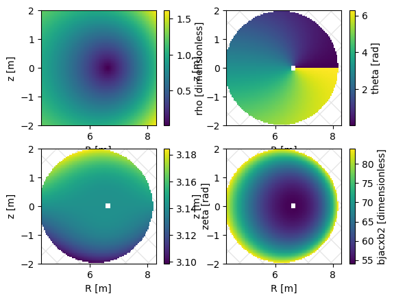
Generating the Boozer coordinates near axis or separatrix may encounter issues, which is why it is a good idea to use the limits rhomin and rhomax to control what area the coordinates cover. Outside this area the MHD input is not evaluated so this it only needs to cover the region where the modes are active, and limiting the region decreases the CPU time needed to run the simulation.

Now let’s plot the \(q\)-profile before generating the MHD input.

rho = np.linspace(0,1,100)
q, I, g = a5.input_eval_safetyfactor(rho)
plt.plot(rho, q)

np.interp(7/4,q,rho)

np.float64(0.4257874821630061)

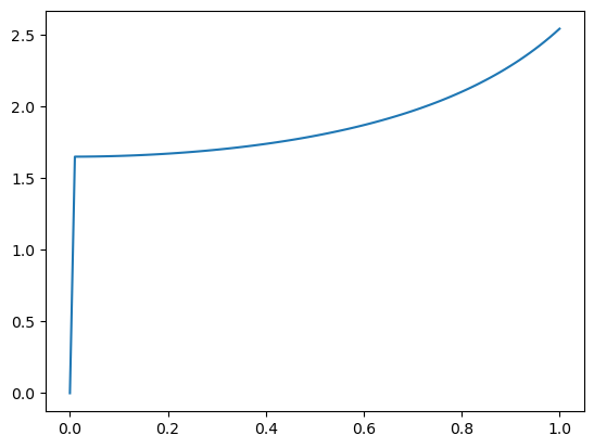
Notice that the q-profile is ill-defined close to the axis, which is caused by the same issue that prevents creation of the Boozer coordinates at that point.

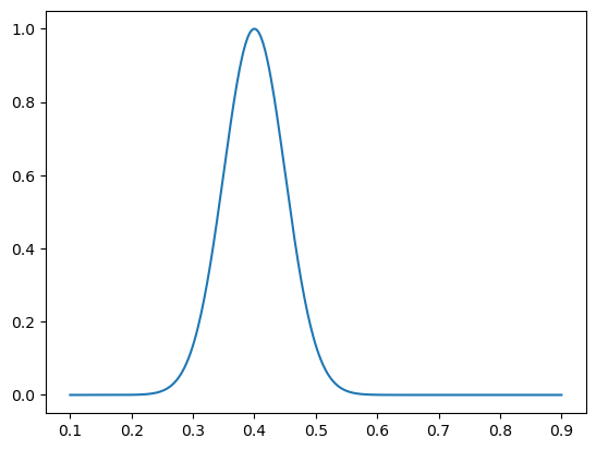
There is rational \(q=7/4\) surface around \(\rho=0.4\), which is where we initialize our MHD mode. Multiple modes can be included in a simulation and they can have time-dependent eigenmodes (though those increase CPU cost considerably). However, for this tutorial we initialize justa a single \((n=4,m=7)\) mode that peaks at the rational surface.

mhd = {
    "nmode" : 1, # Number of modes
    "nmodes" : np.array([4]), "mmodes" : np.array([7]), # Mode tor and pol numbers
    "amplitude" : np.array([1.0]), "omega" : np.array([50.0e6]), "phase" : np.array([0.0]),
    "nrho" : 500, "rhomin" : 0.1, "rhomax" : 0.9
   }

# Eigenmodes are given in the usual sqrt of normalized poloidal flux grid
rhogrid = np.linspace(mhd["rhomin"], mhd["rhomax"], mhd["nrho"])
alpha   = np.exp( -(rhogrid-0.4)**2/0.005 ) # Magnetic potential
phi     = alpha*0 # Electric perturbation potential, we will come back to this

mhd["phi"]   = np.tile(phi,   (mhd["nmode"],1)).T
mhd["alpha"] = np.tile(alpha, (mhd["nmode"],1)).T
a5.data.create_input("MHD_STAT", **mhd, desc="UNSCALED")

plt.figure()
plt.plot(rhogrid, alpha)
plt.show()

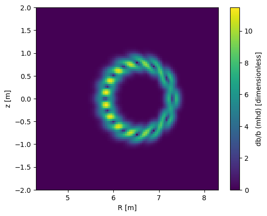
We used the tag “UNSCALED” for this input to notify that it is not suitable for a simulation yet. When using data provided by other codes, the MHD input is usually unscaled meaning that the eigenmodes are otherwise fine, but they have to be scaled by the amplitude parameter so that we get the desired perturbation level \(\delta B/B\).

So now let’s initialize the MHD input and plot the perturbation level.

# Note that plotting MHD requires that both bfield and boozer are also initialized
# but those we have initialized earlier in this tutorial.
a5.input_init(mhd=a5.data.mhd.UNSCALED.get_qid())
a5.input_plotrz(rgrid, zgrid, "db/b (mhd)")
a5.input_free(mhd=True)

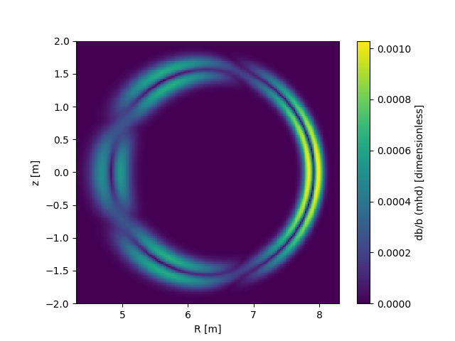
For this tutorial, we desire something like \(\delta B/B \approx 10^{-3}\). Let’s read the input and fix the amplitude:

mhd = a5.data.mhd.UNSCALED.read()
mhd["amplitude"][:] = 1e-3 / 8.1

a5.data.create_input("MHD_STAT", **mhd, desc="SCALED")
a5.input_init(mhd=a5.data.mhd.SCALED.get_qid())
a5.input_plotrz(rgrid, zgrid, "db/b (mhd)")

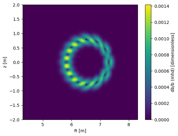
Better!

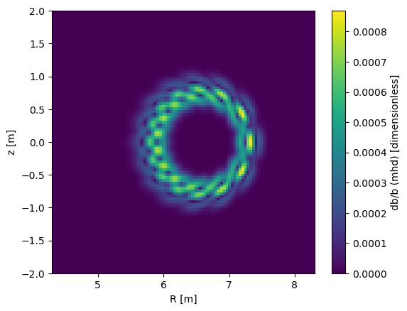
The electric perturbation potential \(\Phi\) will be scaled by the same amplitude. So far in this tutorial we have had \(\Phi=0\), which of course is usually not the case in real life, though ASCOT5 can be run with just the magnetic perturbation or vice versa.

Sometimes the physics dictate that \(E_\parallel=0\), which makes \(\alpha_{nm}\) and \(\Phi_{nm}\) codependent:

\[\omega_{nm}\alpha_{nm} = \frac{nq-m}{I+gq}\Phi_{nm}.\]

There is an existing tool that uses this relation to compute \(\Phi_{nm}\) from \(\alpha_{nm}\) (or vice-versa). However, since \(\alpha\) in this tutorial is arbitrary, calculating \(\Phi\) from it would have divergence issues on a rational surface (where \(nq-m=0\) but \(\alpha_nm \neq 0\)). What we do instead is that we first choose a \(\Phi\) profile, then calculate \(\alpha\) as this way the divergence is not an issue, and then scale the modes.

# Switch Phi and alpha profiles and calculate new alpha from Phi assuming Epar=0
mhd = a5.data.mhd.SCALED.read()
mhd["phi"] = mhd["alpha"]
mhd = a5.data.create_input("mhd consistent potentials", mhd=mhd,
        which="alpha", desc="ZEROEPARUNSCALED", dryrun=True)

# Scale amplitudes to obtain dB/B ~ 1e-3
mhd["amplitude"][:] = 2e6

# Plot dB/B
a5.data.create_input("MHD_STAT", **mhd, activate=True, desc="ZEROEPAR")
a5.input_init(mhd=True, switch=True)
a5.input_plotrz(rgrid, zgrid, "db/b (mhd)")

One can of course provide \(\Phi_{nm}\) explicitly, even when \(E_\parallel=0\), and it is advised to do so when both are available.

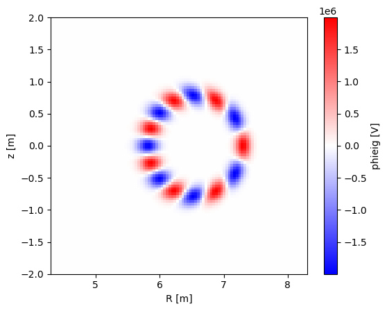
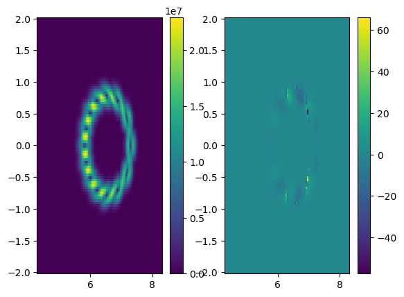
Now to verify that \(E_\parallel=0\), which should be done when the potentials are provided by a code that enforces this condition to ensure the data was imported (and Boozer coordinates constructed) succesfully:

a5.input_plotrz(rgrid, zgrid, "phieig")

phi   = 0*unyt.deg
t     = 0*unyt.s
br, bphi, bz, er, ephi, ez = a5.input_eval(
    rgrid, phi, zgrid, t, "br", "bphi", "bz", "mhd_er", "mhd_ephi", "mhd_ez", grid=True)

bnorm = np.squeeze(np.sqrt(br**2 + bphi**2 + bz**2))
enorm = np.squeeze(np.sqrt(er**2 + ephi**2 + ez**2))
epar  = np.squeeze(br*er + bphi*ephi + bz*ez) / bnorm

fig = plt.figure()
ax = fig.add_subplot(1,2,1)
h = ax.pcolormesh(rgrid, zgrid, enorm.T)
plt.colorbar(h, ax=ax)
ax = fig.add_subplot(1,2,2)
h = ax.pcolormesh(rgrid, zgrid, epar.T)
plt.colorbar(h, ax=ax)
plt.show()

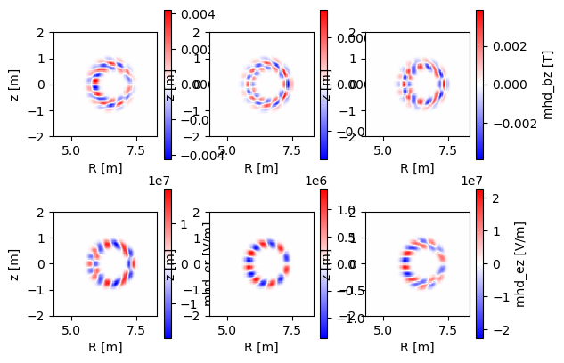
The following visualizes all components of the MHD perturbation:

fig = plt.figure()
ax = fig.add_subplot(2,3,1)
a5.input_plotrz(rgrid, zgrid, "mhd_br", axes=ax)
ax = fig.add_subplot(2,3,2)
a5.input_plotrz(rgrid, zgrid, "mhd_bphi", axes=ax)
ax = fig.add_subplot(2,3,3)
a5.input_plotrz(rgrid, zgrid, "mhd_bz", axes=ax)
ax = fig.add_subplot(2,3,4)
a5.input_plotrz(rgrid, zgrid, "mhd_er", axes=ax)
ax = fig.add_subplot(2,3,5)
a5.input_plotrz(rgrid, zgrid, "mhd_ephi", axes=ax)
ax = fig.add_subplot(2,3,6)
a5.input_plotrz(rgrid, zgrid, "mhd_ez", axes=ax)
plt.show()

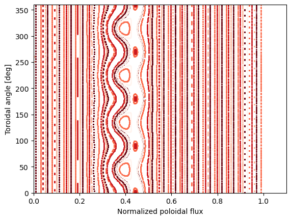
As a final check, we generate Poincaré plots for this data. (The details of generating Poincaré plots are covered in a separate tutorial.) When setting Poincaré options, we need to switch mhd=True which activates ENABLE_MHD in the simulation options, which in turn includes the MHD contribution to the orbit-following.

Poincaré plots can be generated for both field lines and particles. There are two notable differences on how these include MHD:

1. Field-line simulations are performed for a frozen perturbation; the mode doesn’t rotate during the simulation so the Poincaré is a snapshot of the field structure. For particle simulations the mode rotates as usual.

2. Field-line (and gyro-orbit) simulations evaluate the perturbed components \(\delta B\) and \(\delta E\) explicitly when integrating the equations of motion. The guiding-center simulations on the other hand evaluates just the potentials \(\alpha\) and \(\Phi\) which are directly included into equations of motion.

The second bullet should have no practical differences, but if gyro-orbit and guiding-center results differ, this information might help in investigating the cause if the result is unexpected.

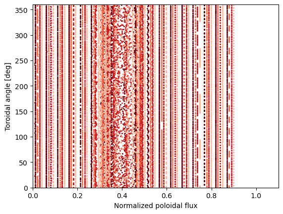
The first bullet explains why for a single mode there are islands in the Poincaré plot and for the particles there is a ergodic region in the same are where the mode has a rational surface:

# Field line Poincare
a5.simulation_initinputs()
mrk = a5.data.create_input("marker poincare", dryrun=True)
opt = a5.data.create_input("options poincare", maxrho=True, mhd=True, dryrun=True)
a5.simulation_initmarkers(**mrk)
a5.simulation_initoptions(**opt)
vrun = a5.simulation_run()
vrun.plotorbit_poincare("tor 1")
a5.simulation_free(markers=True, diagnostics=True)

# Alpha particle Poincare
mrk = a5.data.create_input("marker poincare", species="alpha", energy=3.5e6, pitch=0.9,
                           dryrun=True)
opt = a5.data.create_input("options poincare", maxrho=True, mhd=True, simmode=2,
                           dryrun=True)
a5.simulation_initmarkers(**mrk)
a5.simulation_initoptions(**opt)
vrun = a5.simulation_run()
vrun.plotorbit_poincare("tor 1")
a5.simulation_free(markers=True, diagnostics=True)

Summary of results:
       99 markers had end condition Max toroidal orbits
        1 markers had end condition Max rho

          No markers were aborted.

Now that the MHD input is thoroughly reviewed, we can run an actual simulation. Once both Boozer and MHD input is present, it is sufficient to toggle ENABLE_MHD in the simulation options. For this tutorial we just trace a single marker without collisions for a few orbits so that we can perform one final check.

from a5py.ascot5io.options import Opt
opt = Opt.get_default()
opt.update({
    "SIM_MODE":2, "FIXEDSTEP_USE_USERDEFINED":1, "FIXEDSTEP_USERDEFINED":1e-8,
    "ENDCOND_SIMTIMELIM":1, "ENDCOND_MAX_MILEAGE":1e-5,
    "ENABLE_ORBIT_FOLLOWING":1, "ENABLE_MHD":1,
    "ENABLE_ORBITWRITE":1, "ORBITWRITE_MODE":1,
    "ORBITWRITE_INTERVAL":1e-8, "ORBITWRITE_NPOINT":10**3,
})

from a5py.ascot5io.marker import Marker
mrk = Marker.generate("gc", n=2, species="alpha")
mrk["energy"][:] = 3.5e6
mrk["pitch"][:]  = [0.5, 0.9]
mrk["zeta"][:]   = 0.0
mrk["r"][:]      = [7.2, 7.3]
mrk["z"][:]      = 0.0
mrk["phi"][:]    = 0.0

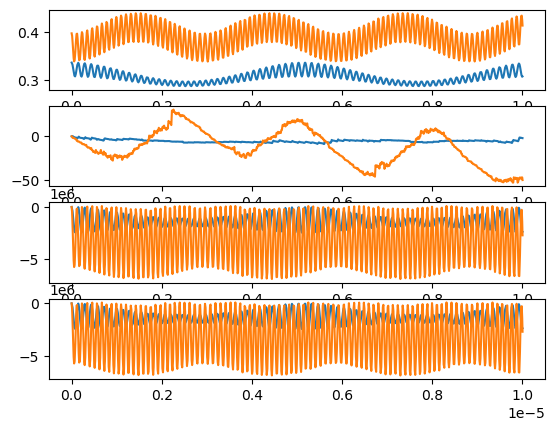
When collisions are disabled and the perturbation consists of a single mode, there is a quantity \(K=H-\omega P / n\), where \(H\) is the Hamiltonian and \(P\) is the toroidal canonical angular momentum, which is conserved. This is true even though the conservation of \(H\) and \(P\) are independently violated. Since we had orbit-diagnostics enabled, we can plot the change in time but for a large number of markers it is sufficient to check this Of course actual simulations may consists of several toroidal modes, but performing this check for the dominant mode increases the confidence that the data was imported succesfully.

a5.simulation_initmarkers(**mrk)
a5.simulation_initoptions(**opt)
vrun = a5.simulation_run()

mhd = a5.data.mhd.ZEROEPAR.read()
ekin, charge, ptor, bphi, r, phi, z, t, ids, rho = vrun.getorbit(
    "ekin", "charge", "ptor", "bphi", "r", "phi", "z", "time", "ids", "rho")
a5.simulation_free()

Phi, alpha = a5.input_eval(r, phi, z, t, "phieig", "alphaeig")

# Can. tor. ang. momentum and Hamiltonian including MHD perturbation
Ptor = ptor + r * charge * alpha * bphi
H = ekin + Phi * charge
P = ( (mhd["omega"]/unyt.s) * Ptor / mhd["nmodes"] ).to("eV")
K = H - P

fig = plt.figure()
ax1 = fig.add_subplot(4,1,1)
ax2 = fig.add_subplot(4,1,2)
ax3 = fig.add_subplot(4,1,3)
ax4 = fig.add_subplot(4,1,4)

ax1.plot(t[ids==1], rho[ids==1], color="C0")
ax1.plot(t[ids==2], rho[ids==2], color="C1")

ax2.plot(t[ids==1], K[ids==1] - K[ids==1][0], color="C0")
ax2.plot(t[ids==2], K[ids==2] - K[ids==2][0], color="C1")

ax3.plot(t[ids==1], H[ids==1] - H[ids==1][0], color="C0")
ax3.plot(t[ids==2], H[ids==2] - H[ids==2][0], color="C1")

ax4.plot(t[ids==1], P[ids==1] - P[ids==1][0], color="C0")
ax4.plot(t[ids==2], P[ids==2] - P[ids==2][0], color="C1")
plt.show()

Summary of results:
       86 markers had end condition Max toroidal orbits
        4 markers had end condition Max poloidal orbits
       10 markers had end condition Max rho

          No markers were aborted.

Summary of results:
        2 markers had end condition Sim time limit

          No markers were aborted.