Dealing with distributions

Notes about distributions and moments in ASCOT5

ASCOT5 is a kinetic code that solves the Fokker-Planck equation indirectly by tracing weighted markers that form the test particle distribution function. Therefore distribution (histograms), which ASCOT5 collects and which approximate the distribution function, can be considered as the main output of the code. In this example we show how to collect and post-process the distributions.

The distribution function in ASCOT5 is represented by N-dimensional histograms that divide the entire (preferably) possible phase-space into a finite grid. Every time a marker is advanced in a simulation, the code finds the correct bin in the histogram and increments that by marker weight times time-step length. We implicitly assume that the marker weight is in units of particles/s meaning that the markers represent a constant particle source e.g. alpha particle birth rate. The collected distribution therefore is a steady-state distribution and it has units of particles.

The distribution function contains all information there is to know about a physical system. Often the distribution function itself is of little interest, and the interesting quantities are the moments of the distribution. While the distribution function is collected during the simulation, the moments are calculated in post-processing.

NOTE: The resolution of the distribution histogram directly affects the accuracy of the calculated moment(s). It is therefore advised to allocate as much memory for the distribution that is available and can be reasonably post-processed.

ASCOT5 can be used to collect following distributions, which can be collected simultaneously in a simulation:

• 5D \((R,\phi,z,p_\parallel,p_\perp)\)

• rho5D \((\rho,\theta,\phi,p_\parallel,p_\perp)\)

• 6D \((R,\phi,z,p_R,p_\phi,p_z)\)

• rho6D \((\rho,\theta,\phi,p_R,p_\phi,p_z)\)

• COM \((E_\mathrm{kin},P_\mathrm{ctor},\mu)\)

5D and rho5D are the default distributions and also the ones that should be used in all guiding-center and hybrid simulations. Both distributions can be used in post-processing to evaluate moments of the distribution, but the difference between these two is that only rho5D can be used to evaluate 1D quantities.

6D and rho6D cannot be used to evaluate moments. They are to be used only in gyro-orbit simulations where the particle distribution on itself is of interest: e.g. for marker sampling.

COM (constant-of-motion) distribution collects the data in kinetic energy, canonical toroidal angular momentum, and magnetic moment coordinates. It cannot be used to compute moments and it is used to provide input from ASCOT5 to other codes.

All distributions except for COM also have additional abscissae in time and charge. Usually these are of little intereset, but make sure to set the charge abscissa properly so that it has a single bin for each expected charge state as otherwise the moments cannot be computed properly.

Summary: Use 5D or rho5D distribution for guiding center simulations and in any simulations where you wish to calculate moments in post-processing. For computing 1D profiles and moments, use rho5D. Use 6D or rho6D in gyro-orbit simulations when the particle distribution is of specific interest. If you need the COM distribution, you’ll know it.

Collecting and plotting distributions

Let’s begin by setting up a test case that mimics alpha particle slowing down:

import numpy as np
import unyt
import matplotlib.pyplot as plt
from a5py import Ascot

a5 = Ascot("ascot.h5", create=True)
a5.data.create_input("bfield analytical iter circular")
a5.data.create_input("plasma flat", density=1e21)
a5.data.create_input("wall_2D")
a5.data.create_input("E_TC")
a5.data.create_input("N0_1D")
a5.data.create_input("Boozer")
a5.data.create_input("MHD_STAT")
a5.data.create_input("asigma_loc")

from a5py.ascot5io.marker import Marker
nmrk = 1000
mrk = Marker.generate("gc", n=nmrk, species="alpha")
mrk["energy"][:] = 3.5e6
mrk["pitch"][:]  = 0.99 - 1.98 * np.random.rand(nmrk,)
mrk["r"][:]      = 4.5 + 3 * np.random.rand(nmrk,)
a5.data.create_input("gc", **mrk)

from a5py.ascot5io.options import Opt
opt = Opt.get_default()
opt.update({
    "SIM_MODE":2, "ENABLE_ADAPTIVE":1,
    "ENDCOND_ENERGYLIM":1, "ENDCOND_MIN_ENERGY":2.0e3, "ENDCOND_MIN_THERMAL":2.0,
    "ENABLE_ORBIT_FOLLOWING":1, "ENABLE_COULOMB_COLLISIONS":1,
})

print("Inputs created")

Inputs created

The principle of setting up distribution data collection is the same for all distributions, so here we only collect 5D and rho5D as those will be used to calculate moments later on. Distributions are very memory intensive so while multiple distributions can be collected simultaneously, it is not always feasible to do so.

opt.update({
    # Distribution output
    "ENABLE_DIST_5D":1, "ENABLE_DIST_RHO5D":1,
    # (R,z) abscissae for the 5D distribution
    "DIST_MIN_R":4.3,  "DIST_MAX_R":8.3, "DIST_NBIN_R":50,
    "DIST_MIN_Z":-2.0, "DIST_MAX_Z":2.0, "DIST_NBIN_Z":50,
    # (rho, theta) abscissae for the rho5D distribution. Most of the time a single
    # theta slot is sufficient but please verify it in your case.
    "DIST_MIN_RHO"  :0, "DIST_MAX_RHO"  :1.0, "DIST_NBIN_RHO"  :100,
    "DIST_MIN_THETA":0, "DIST_MAX_THETA":360, "DIST_NBIN_THETA":1,
    # Single phi slot since this is not a stellarator.
    # These values are shared between other distributions
    "DIST_MIN_PHI":0,        "DIST_MAX_PHI":360,     "DIST_NBIN_PHI":1,
    # The momentum abscissae are shared by 5D distributions
    "DIST_MIN_PPA":-1.3e-19, "DIST_MAX_PPA":1.3e-19, "DIST_NBIN_PPA":100,
    "DIST_MIN_PPE":0,        "DIST_MAX_PPE":1.3e-19, "DIST_NBIN_PPE":50,
    # One time slot, the span doesn't matter as long as it covers the whole simulation time
    "DIST_MIN_TIME":0,       "DIST_MAX_TIME":1.0,    "DIST_NBIN_TIME":1,
    # One charge slot exactly at q=2 since we are simulating alphas
    "DIST_MIN_CHARGE":1.5,   "DIST_MAX_CHARGE":2.5,    "DIST_NBIN_CHARGE":1,
})
a5.data.create_input("opt", **opt)

'opt_0273630877'

Now run the simulation.

import subprocess
subprocess.run(["./../../build/ascot5_main", "--d=\"SDALPHA\""])
print("Simulation completed")

ASCOT5_MAIN
Tag cc4ce10
Branch docs

Initialized MPI, rank 0, size 1.

Reading and initializing input.

Input file is ascot.h5.

Reading options input.
Active QID is 0273630877
Options read and initialized.

Reading magnetic field input.
Active QID is 0367928479

Analytical tokamak magnetic field (B_GS)
Psi at magnetic axis (6.618 m, -0.000 m)
-5.410 (evaluated)
-5.410 (given)
Magnetic field on axis:
B_R = 0.000 B_phi = 4.965 B_z = -0.000
Number of toroidal field coils 0
Estimated memory usage 0.0 MB
Magnetic field read and initialized.

Reading electric field input.
Active QID is 2105262353

Trivial Cartesian electric field (E_TC)
E_x = 0.000000e+00, E_y = 0.000000e+00, E_z = 0.000000e+00
Estimated memory usage 0.0 MB
Electric field read and initialized.

Reading plasma input.
Active QID is 0441992228

1D plasma profiles (P_1D)
Min rho = 0.00e+00, Max rho = 1.00e+01, Number of rho grid points = 100, Number of ion species = 1
Species Z/A  charge [e]/mass [amu] Density [m^-3] at Min/Max rho    Temperature [eV] at Min/Max rho
   1  /  1     1  /  1.000             1.00e+21/1.00e+00                1.00e+04/1.00e+04
[electrons]   -1  /  0.001             1.00e+21/1.00e+00                1.00e+04/1.00e+04
Quasi-neutrality is (electron / ion charge density) 1.00
Estimated memory usage 0.0 MB
Plasma data read and initialized.

Reading neutral input.
Active QID is 0461643578

1D neutral density and temperature (N0_1D)
Grid:  nrho =    3   rhomin = 0.000   rhomax = 2.000
 Number of neutral species = 1
Species Z/A   (Maxwellian)
        1/  1 (1)
Estimated memory usage 0.0 MB
Neutral data read and initialized.

Reading wall input.
Active QID is 0480419459

2D wall model (wall_2D)
Number of wall elements = 4, R extend = [0.01, 100.00], z extend = [-100.00, 100.00]
Estimated memory usage 0.0 MB
Wall data read and initialized.

Reading boozer input.
Active QID is 1655620106

Boozer input
psi grid: n =    6 min = 0.000 max = 1.000
thetageo grid: n =   18
thetabzr grid: n =   10
Boozer data read and initialized.

Reading MHD input.
Active QID is 3727342173

MHD (stationary) input
Grid: nrho =    6 rhomin = 0.000 rhomax = 1.000

Modes:
(n,m) = ( 1, 3) Amplitude = 0.1 Frequency =   1 Phase =   0
(n,m) = ( 2, 4) Amplitude =   2 Frequency = 1.5 Phase = 0.785
Estimated memory usage 0.0 MB
MHD data read and initialized.

Reading atomic reaction input.
Active QID is 0597020235

Found data for 1 atomic reactions:
Reaction number / Total number of reactions = 1 / 1
  Reactant species Z_1 / A_1, Z_2 / A_2     = 1 / 1, 1 / 1
  Min/Max energy                            = 1.00e+03 / 1.00e+04
  Min/Max density                           = 1.00e+18 / 1.00e+20
  Min/Max temperature                       = 1.00e+03 / 1.00e+04
  Number of energy grid points              = 3
  Number of density grid points             = 4
  Number of temperature grid points         = 5
Estimated memory usage 0.0 MB
Atomic reaction data read and initialized.

Reading marker input.
Active QID is 0224444363

Loaded 1000 guiding centers.
Marker data read and initialized.

All input read and initialized.

Initializing marker states.
Estimated memory usage 0.0 MB.
Marker states initialized.
Initialized diagnostics, 99.2 MB.

Preparing output.
Note: Output file ascot.h5 is already present.

The qid of this run is 1415480022

Inistate written.
Simulation begins; 4 threads.
Simulation complete.
Simulation finished in 96.246512 s
Endstate written.

Combining and writing diagnostics.

Writing diagnostics output.

Writing 5D distribution.

Writing rho 5D distribution.

Diagnostics output written.
Diagnostics written.

Summary of results:
     1000 markers had end condition Thermalization

          No markers were aborted.

Done.
Simulation completed

Distributions are accessed via getdist method that returns a DistData object which contains methods for additional processing and plotting. The data can be sliced, integrated, and interpolated. For plotting, the distribution must be reduced to 2D or 1D first.

a5 = Ascot("ascot.h5")
dist = a5.data.active.getdist("5d")

print("List of abscissae:")
print(dist.abscissae)

# Abscissa values (bin center points)
dist.abscissa("r");
# Bin edges
dist.abscissa_edges("r");
# Value of the distribution function
dist.distribution();
# Phase-space volume of bin elements
dist.phasespacevolume();
# Number of particles per bin (= distribution x phasespacevolume)
dist.histogram();

# Perform linear interpolation on R at the given value
dist.interpolate(r=6.6*unyt.m);

# Take a slice by giving <name of the abscissa>=<indices to be sliced>
dist.slice(r=np.s_[1:-1])

# Slicing and integrating modifies the distribution object, unless copy=True is given
dist.integrate(phi=np.s_[:], charge=np.s_[:], time=np.s_[:])

rzdist = dist.integrate(copy=True, ppar=np.s_[:], pperp=np.s_[:])
dist.integrate(r=np.s_[:], z=np.s_[:], pperp=np.s_[:])

rzdist.plot()
dist.plot()

List of abscissae:
['r', 'phi', 'z', 'ppar', 'pperp', 'time', 'charge']

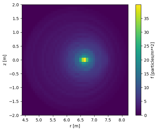
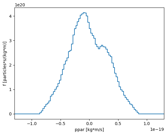
Note that the units of the distribution, \(f\), remain consistent when the operations above are used.

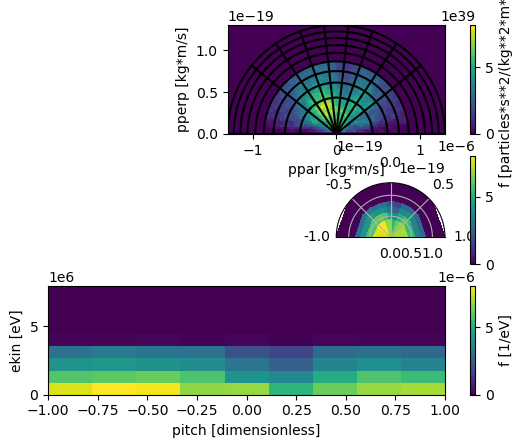
The momentum space in 5D distributions can also be converted to energy and pitch, \((E_\mathrm{kin},\xi)\), which can be more convenient to use. The resulting DistData object is no different, except that it can’t be used to evaluate moments. Setting plotexi=True visualizes the transformation: the top plot shows the original momentum space with the new grid overlayed, the second plot shows the distribution after rebinning, and the third shows the final distribution in the new basis.

distexi = a5.data.active.getdist("5d", ekin_edges=10, pitch_edges=10, exi=True, plotexi=True)

# Integrate over all dimensions to get the total particle number
distexi.integrate(r=np.s_[:],phi=np.s_[:],z=np.s_[:],ekin=np.s_[:],pitch=np.s_[:],
                  charge=np.s_[:],time=np.s_[:])
dist = a5.data.active.getdist("5d")
dist.integrate(r=np.s_[:],phi=np.s_[:],z=np.s_[:],ppar=np.s_[:],pperp=np.s_[:],
               charge=np.s_[:],time=np.s_[:])
print("Particle numbers are %e and %e" % (dist.histogram(), distexi.histogram()))

Particle numbers are 3.299464e+01 and 3.299464e+01

The conversion basically “re-bins” the histogram thus preserving the total particle number. The resolution of the new momentum space should be similar to the one in \((p_\parallel,p_\perp)\). If it is significantly higher, “holes” can appear in the distribution.

distexi = a5.data.active.getdist("5d", ekin_edges=50, pitch_edges=50, exi=True)
distexi.integrate(r=np.s_[:],phi=np.s_[:],z=np.s_[:],charge=np.s_[:],time=np.s_[:])
distexi.plot()

Moments

Moments are computed from the DistData object, so it is possible to process the data before it is passed to getdist_moments which computes the moments. The result is a DistMoment object:

# Evaluate moment by giving the distribution and specifying what moment is to be evaluated
dist = a5.data.active.getdist("5d")
mom2d = a5.data.active.getdist_moments(dist, "density")

# Moment object integrates over all momentum space (and time and charge) so that in the end
# it stores the data in 3D spatial grid and it records physical volume and poloidal area of each bin
mom2d.volume;
mom2d.area;

# Grid center (R,phi,z coordinates)
mom2d.rc;
mom2d.phic;
mom2d.zc;

# The value is stored as an ordinate and accessed like this
# This returns (nr,nphi,nz) matrix.
mom2d.ordinate("density");

# Multiple moments can be evaluated simultaneously
mom2d = a5.data.active.getdist_moments(dist, "density", "chargedensity")

# Single object can store multiple moments, which can be listed like this
print("Stored moments")
print(mom2d.list_ordinates())

# All available distributions and moments that can be calculated
a5.data.active.getdist_list();

# Evaluating some distributions requires interpolating input data
a5.input_init(bfield=True)
a5.data.active.getdist_moments(dist, "parallelcurrent")
a5.input_free()

Stored moments
['density', 'chargedensity']
Available distributions:
5d
rho5d
Available Moments:
density : Particle number density
chargedensity : Charge density
energydensity : Energy density
toroidalcurrent : Toroidal current
parallelcurrent : Parallel current
pressure : Pressure
powerdep : Total deposited power
ionpowerdep : Power deposited to ions
electronpowerdep : Power deposited to electrons

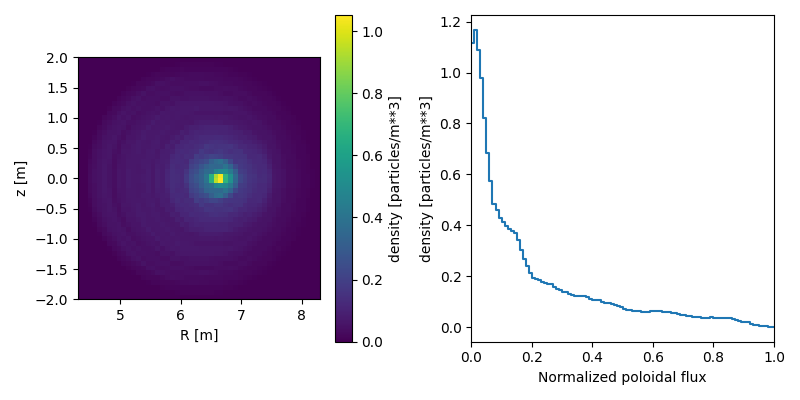
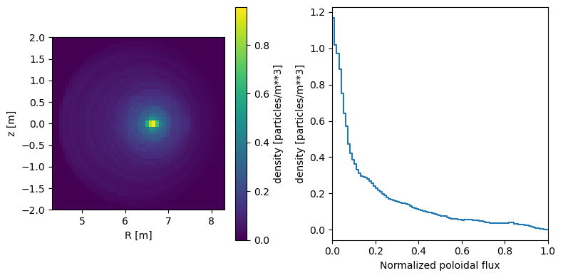
DistMoment behaves differently depending on whether it was calculated from 5d or rho5d distribution. The abscissae are different and for 5d one can take a toroidal average of the moment and for rho5d both toroidal and poloidal averages are possible. The average values are used when plotting the moments.

dist = a5.data.active.getdist("5d")
mom2d = a5.data.active.getdist_moments(dist, "density")

# Evaluating moments from rho5d always requires bfield initialization so
# that (rho,theta) can be mapped to (r,z)
dist = a5.data.active.getdist("rho5d")
a5.input_init(bfield=True)
mom1d = a5.data.active.getdist_moments(dist, "density")
a5.input_free()

# Moment objects have different abscissae
mom1d.rho;
mom1d.theta;
mom1d.phi;
mom2d.r;
mom2d.phi;
mom2d.z;

# Poloidal average only valid for moments calculated from rho5d
mom2d.ordinate("density", toravg=True);
mom1d.ordinate("density", toravg=True, polavg=True);

fig = plt.figure(figsize=(8,4))
ax1 = fig.add_subplot(1,2,1)
ax2 = fig.add_subplot(1,2,2)

mom2d.plot("density", axes=ax1)
mom1d.plot("density", axes=ax2)

plt.tight_layout()
plt.show()

Distribution resolution must be chosen carefully since moments are calculated in post-processing and there is a loss of information when the markers are binned to the histogram. Running even a short simulation with different distribution settings helps finding the correct values.

Other possible source of error is the volume calculation, for moments computed from rho5d, which is also done in post-processing. There are two methods to compute the volume and it is always good to check that those agree.

a5.input_init(bfield=True)
# Divide volume into prisms and sum them
mom1 = a5.data.active.getdist_moments(dist, "density", volmethod="prism")
# Calculate volume using Monte Carlo method
mom2 = a5.data.active.getdist_moments(dist, "density", volmethod="mc")
a5.input_free()

print(np.sum(mom1.volume))
print(np.sum(mom2.volume))

/home/runner/work/ascot5/ascot5/a5py/ascotpy/__init__.py:955: AscotUnitWarning: Argument(s) theta given without dimensions (assumed rad)
  rc, zc = self.input_rhotheta2rz(

489.52620062954577 m**3
489.5201219456913 m**3