Modelling CX and tracing neutrals
This example shows how to include atomic reactions that change the charge state of the markers, and how to model neutrals.
NOTE: This tutorial requires ADAS data to run. Therefore the results won’t be displayed on the online version.
At its current state, the atomic physics in ASCOT5 enables simulation of neutrals and singly charged ions. Neutral can become ionized and ion can become neutral but it is not currently possible for ion to remain ion when its charge state changes.
We begin by creating some test data that is not directly relevant for this tutorial.
[1]:
import numpy as np
import unyt
import matplotlib.pyplot as plt
from a5py import Ascot

a5 = Ascot("ascot.h5", create=True)
a5.data.create_input("bfield analytical iter circular")
a5.data.create_input("wall rectangular")
a5.data.create_input("E_TC")
a5.data.create_input("Boozer")
a5.data.create_input("MHD_STAT")

print("Inputs created")
/home/runner/work/ascot5/ascot5/a5py/routines/plotting.py:35: UserWarning: Could not import cKDTree and alphashape. 3D surface plotting disabled.
  warnings.warn(
Inputs created
As for the plasma and neutral data, pay attention to the following:
Plasma species must be fully ionized, i.e.
chargeandznummust match (partially ionized species have not been implemented yet).The neutral species must be in the same order as the species in the plasma input (neutral data does not yet contain
anumandznumfields so the ones in the plasma input are used instead).
In this tutorial we have \(^1_1\)H plasma and neutrals.
[2]:
# Plasma data
nrho   = 11
rho    = np.linspace(0, 2, nrho).T
vtor   = np.zeros((nrho, 1))
edens  = 1e18 * np.ones((nrho, 1))
etemp  = 1e3  * np.ones((nrho, 1))
idens  = 1e18 * np.ones((nrho, 1))
itemp  = 1e3  * np.ones((nrho, 1))

pls = {
    "nrho" : nrho, "nion" : 1, "rho" : rho, "vtor": vtor,
    "anum" : np.array([2]), "znum" : np.array([1]),
    "mass" : np.array([1.007]), "charge" : np.array([1]),
    "edensity" : edens, "etemperature" : etemp,
    "idensity" : idens, "itemperature" : itemp}
a5.data.create_input("plasma_1D", **pls, desc="FLAT")

# Neutral data
density = np.ones((11,1)) * 1e17
temperature = np.ones((11,1)) * 1e3
ntr = {"rhomin" : 0, "rhomax" : 10, "nrho" : 11, "nspecies" : 1,
       "anum" : np.array([1]), "znum" : np.array([1]),
       "density" : density, "temperature" : temperature,
       "maxwellian" : 1}
a5.data.create_input("N0_1D", **ntr, desc="FLAT")
[2]:
'N0_1D_2253930496'
When generating the marker input, note that anum and znum fields specify the particle species whereas charge specifies the charge state. One can assume that the mass is same for all charge states and it stays fixed in the simulation. For this tutorial we create equal amounts of ions and neutrals.
[3]:
from a5py.ascot5io.marker import Marker
mrk = Marker.generate("gc", n=100, species="deuterium")
mrk["energy"][:] = 1.0e4
mrk["pitch"][:]  = 0.99 - 1.98 * np.random.rand(100,)
mrk["r"][:]      = np.linspace(6.2, 7.2, 100)
mrk["charge"][:50] = 0
mrk["charge"][50:] = 1
a5.data.create_input("gc", **mrk)
[3]:
'gc_0830408443'
Atomic data is created using ADAS or Open-ADAS datasets if those are available. Since these tutorials are run on the GitHub server, we don’t have ADAS available and we have to resort to analytical models.
[4]:
try:
    a5.data.create_input("import_adas")
except Exception as err:
    print(err)
    print("Using analytical model instead.")
    a5.data.create_input("asigma_chebyshev_cx_hh0")
Could not import adas package.
Using analytical model instead.
Once generated, the atomic data can be interpolated via ascotpy. Now we can calculate the mean-free-time which in turn gives us a good estimate on what the simulation time-step should be.
[5]:
# First calculate velocity with physlib
#import a5py.physlib as physlib
from a5py import physlib
gamma = physlib.gamma_energy(mrk["mass"][0], mrk["energy"][0])
vnorm = physlib.vnorm_gamma(gamma)

a5.input_init(bfield=True, plasma=True, neutral=True, asigma=True)
sigmacx  = a5.input_eval_atomiccoefs(
    mrk["mass"][0], mrk["anum"][0], mrk["znum"][0],
    mrk["r"][0], mrk["phi"][0], mrk["z"][0], mrk["time"][0], vnorm,
    reaction="charge-exchange")
sigmabms = a5.input_eval_atomiccoefs(
    mrk["mass"][0], mrk["anum"][0], mrk["znum"][0],
    mrk["r"][0], mrk["phi"][0], mrk["z"][0], mrk["time"][0], vnorm,
    reaction="beamstopping")
a5.input_free()
mft_cx  = 1/sigmacx
mft_bms = 1/sigmabms

print("Mean free time: %.3e (CX) %.3e (BMS)" % (mft_cx[0], mft_bms[0]))
/tmp/ipykernel_3976/481609561.py:20: DeprecationWarning: Conversion of an array with ndim > 0 to a scalar is deprecated, and will error in future. Ensure you extract a single element from your array before performing this operation. (Deprecated NumPy 1.25.)
  print("Mean free time: %.3e (CX) %.3e (BMS)" % (mft_cx[0], mft_bms[0]))
Mean free time: 8.556e-05 (CX) 9.330e-06 (BMS)
Once atomic input data has been created, the physics are enabled from options with ENABLE_ATOMIC=1. However, consider setting ENABLE_ATOMIC=2 when there is a possibility that the marker orbits are outside the separatrix where the temperature and density can be outside the data range in which the atomic data is given. When using ENABLE_ATOMIC=2, the cross sections are set to zero when extrapolating the data. Otherwise the simulation would terminate with an error.
If you wish to terminate the simulation when a marker ionizes or when it becomes neutral, you can enable the end conditions ENDCOND_IONIZED and ENDCOND_NEUTRAL, respectively.
When collecting distributions it is important to set the charge abscissa properly. The abscissa should cover all expected charge states and there should be exactly one bin for each charge state.
Here we set simulation options for tracing markers for a fixed time with atomic reactions and Coulomb collisions enabled. We also collect distribution and orbit data.
Finally, it is important to note that the atomic reactions are implemented only for the gyro-orbit mode, SIM_MODE=1, and it is not possible at all to simulate neutrals in guiding center mode. In SIM_MODE=1, the neutrals are traced according to their ballistic trajectories. However, the marker input can still be either particles or guiding centers as in the latter case the guiding center is transformed to particle coordinates using the zeroth order transformation (where the
gyroradius \(\rho_g=0\)) if the marker is a neutral. Same is done for the ini- and endstate but it is recommended to use the particle coordinates nevertheless.
[6]:
from a5py.ascot5io.options import Opt

opt = Opt.get_default()
opt.update({
    # Simulation mode and end condition (use rho max as otherwise neutral escape from
    # the plasma and become aborted since we don't have a proper wall)
    "SIM_MODE":1, "FIXEDSTEP_USE_USERDEFINED":1, "FIXEDSTEP_USERDEFINED":1e-8,
    "ENDCOND_SIMTIMELIM":1, "ENDCOND_MAX_MILEAGE":1e-4,
    "ENDCOND_RHOLIM":1, "ENDCOND_MAX_RHO":1.0,
    # Physics
    "ENABLE_ORBIT_FOLLOWING":1, "ENABLE_COULOMB_COLLISIONS":1, "ENABLE_ATOMIC":1,
    # Distribution output
    "ENABLE_DIST_RHO5D":1,
    "DIST_MIN_RHO":0.0,      "DIST_MAX_RHO":1.0,     "DIST_NBIN_RHO":50,
    "DIST_MIN_PHI":0,        "DIST_MAX_PHI":360,     "DIST_NBIN_PHI":1,
    "DIST_MIN_THETA":0.0,    "DIST_MAX_THETA":360,   "DIST_NBIN_THETA":1,
    "DIST_MIN_PPA":-1.3e-19, "DIST_MAX_PPA":1.3e-19, "DIST_NBIN_PPA":100,
    "DIST_MIN_PPE":0,        "DIST_MAX_PPE":1.3e-19, "DIST_NBIN_PPE":50,
    "DIST_MIN_TIME":0,       "DIST_MAX_TIME":1.0,    "DIST_NBIN_TIME":1,
    "DIST_MIN_CHARGE":-1,    "DIST_MAX_CHARGE":2,    "DIST_NBIN_CHARGE":2,
    # Orbit output
    "ENABLE_ORBITWRITE":1, "ORBITWRITE_MODE":1,
    "ORBITWRITE_INTERVAL":1e-7, "ORBITWRITE_NPOINT":10**4,
})
a5.data.create_input("opt", **opt, desc="TUTORIAL")
[6]:
'opt_2660339990'
Now let us run the simulation:
[7]:
import subprocess
subprocess.run(["./../../build/ascot5_main"])
print("Simulation completed")
ASCOT5_MAIN
Tag 6290a22
Branch docs

Initialized MPI, rank 0, size 1.

Reading and initializing input.

Input file is ascot.h5.

Reading options input.
Active QID is 2660339990
Options read and initialized.

Reading magnetic field input.
Active QID is 0449985548

Analytical tokamak magnetic field (B_GS)
Psi at magnetic axis (6.618 m, -0.000 m)
-5.410 (evaluated)
-5.410 (given)
Magnetic field on axis:
B_R = 0.000 B_phi = 4.965 B_z = -0.000
Number of toroidal field coils 0
Magnetic field read and initialized.

Reading electric field input.
Active QID is 2424628551

Trivial Cartesian electric field (E_TC)
E_x = 0.000000e+00, E_y = 0.000000e+00, E_z = 0.000000e+00
Electric field read and initialized.

Reading plasma input.
Active QID is 2440304539

1D plasma profiles (P_1D)
Min rho = 0.00e+00, Max rho = 2.00e+00, Number of rho grid points = 11, Number of ion species = 1
Species Z/A  charge [e]/mass [amu] Density [m^-3] at Min/Max rho    Temperature [eV] at Min/Max rho
   1  /  2     1  /  1.007             1.00e+18/1.00e+18                1.00e+03/1.00e+03
[electrons]   -1  /  0.001             1.00e+18/1.00e+18                1.00e+03/1.00e+03
Toroidal rotation [rad/s] at Min/Max rho: 0.00e+00/0.00e+00
Quasi-neutrality is (electron / ion charge density) 1.00
Toroidal rotation [rad/s] at Min/Max rho: 0.00e+00/0.00e+00
Plasma data read and initialized.

Reading neutral input.
Active QID is 2253930496

1D neutral density and temperature (N0_1D)
Grid:  nrho =   11   rhomin = 0.000   rhomax = 10.000
 Number of neutral species = 1
Species Z/A   (Maxwellian)
        1/  1 (1)
Neutral data read and initialized.

Reading wall input.
Active QID is 2302824411

2D wall model (wall_2D)
Number of wall elements = 20, R extend = [4.10, 8.40], z extend = [-3.90, 3.90]
Wall data read and initialized.

Reading boozer input.
Active QID is 3799474652

Boozer input
psi grid: n =    6 min = 0.000 max = 1.000
thetageo grid: n =   18
thetabzr grid: n =   10
Boozer data read and initialized.

Reading MHD input.
Active QID is 1043809149

MHD (stationary) input
Grid: nrho =    6 rhomin = 0.000 rhomax = 1.000

Modes:
(n,m) = ( 1, 3) Amplitude = 0.1 Frequency =   1 Phase =   0
(n,m) = ( 2, 4) Amplitude =   2 Frequency = 1.5 Phase = 0.785
MHD data read and initialized.

Reading atomic reaction input.
Active QID is 2884801672

Found data for 1 atomic reactions:
Reaction number / Total number of reactions = 1 / 1
  Reactant species Z_1 / A_1, Z_2 / A_2     = 1 / 2, 1 / 2
  Min/Max energy                            = 5.00e+01 / 1.50e+05
  Min/Max density                           = 1.00e+00 / 1.00e+30
  Min/Max temperature                       = 1.00e+02 / 1.00e+04
  Number of energy grid points              = 200
  Number of density grid points             = 1
  Number of temperature grid points         = 20
Atomic reaction data read and initialized.

Reading marker input.
Active QID is 0830408443

Loaded 100 guiding centers.
Marker data read and initialized.

All input read and initialized.

Initializing marker states.
Estimated memory usage 0.0 MB.
Marker states initialized.

Preparing output.
Note: Output file ascot.h5 is already present.

The qid of this run is 1677759592

Inistate written.
Simulation begins; 4 threads.
Simulation complete.
Simulation finished in 0.207201 s
Endstate written.

Combining and writing diagnostics.

Writing diagnostics output.

Writing rho 5D distribution.
Writing orbit diagnostics.

Diagnostics output written.
Diagnostics written.

Summary of results:
       72 markers had end condition Max rho
       28 markers had end condition Sim time limit

          No markers were aborted.

Done.
Simulation completed
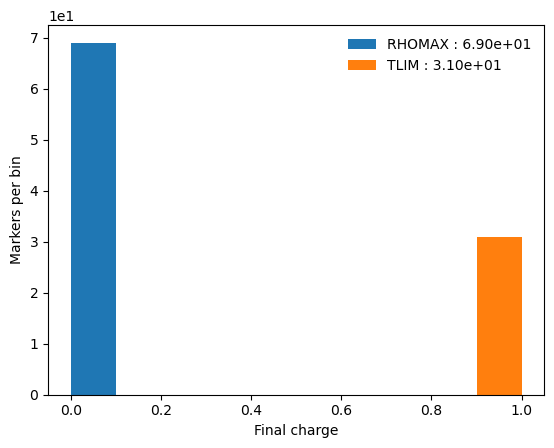
In post-processing we can plot the final charge distribution as
[8]:
a5 = Ascot("ascot.h5")
a5.data.active.plotstate_histogram("end charge")
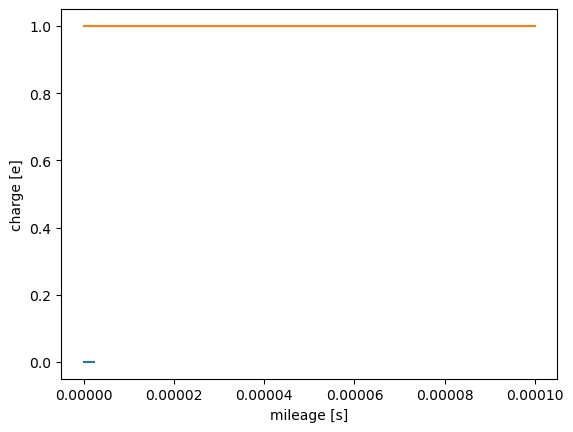
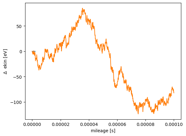
The orbit data contain the marker charge at each time step. Here we verify that the energy has not changed while the marker was neutral since Coulomb collisions only affect charged particles (how well the plot below demonstrates this point depends on RNG).
[9]:
a5.data.active.plotorbit_trajectory("mileage", "charge", ids=[1, 51])
a5.data.active.plotorbit_trajectory("mileage", "diff ekin", ids=[1, 51])
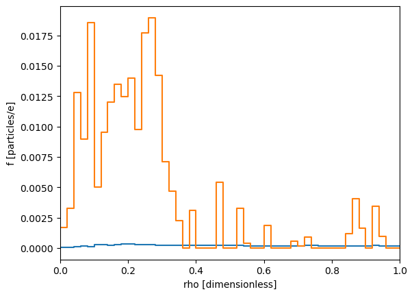
Distributions and moments can be obtained for each charge state separately when the charge abscissa was set properly. Here we plot the neutral and ion densities separately.
[10]:
dist = a5.data.active.getdist("rho5d")
# Integrate over all dimensions except rho and charge
dist.integrate(phi=np.s_[:], theta=np.s_[:], ppar=np.s_[:], pperp=np.s_[:], time=np.s_[:])

# Copy and slice charge at 0 and +1. Then integrate charge so that we can plot
neutraldist = dist.slice(copy=True, charge=0)
dist.slice(charge=1)

fig, ax = plt.subplots()
neutraldist.plot(axes=ax)
dist.plot(axes=ax)
plt.show()