Generating markers
This tutorial illustrates the different ways marker input is created.
Generating markers explicitly
The straight-forward way to initialize markers is to just fill the marker dictionary with proper data. Marker input can either consist of particles, guiding centers, or field lines, but the input does not necessarily have to correspond to the simulation mode. It is perfectly fine to use particle input for a guiding-center simulation and vice-versa. The only real limitation is that field line input can only be used in field line simulations.
NOTE: When particle or guiding center input is used in a field line simulation, the field lines to be traced are initialized at the (particle’s) guiding center position.
You can find the information on what data is required to initialize a specific type of marker in the description of the corresponding write_hdf5 function. A more convenient way is to use a5py.ascot5io.marker.Marker.generate to create an empty template that already contains the relevant arrays where you only need to replace the dummy values with actual data:
[1]:
import numpy as np
import matplotlib.pyplot as plt
import unyt
from a5py.ascot5io.marker import Marker
mrk = Marker.generate("gc", n=100)
mrk["energy"][:] = 3.5e6
mrk["pitch"][:]  = 0.99 - 1.98 * np.random.rand(100,)
mrk["r"][:]      = np.linspace(6.2, 8.2, 100)
/home/runner/work/ascot5/ascot5/a5py/routines/plotting.py:35: UserWarning: Could not import cKDTree and alphashape. 3D surface plotting disabled.
  warnings.warn(
It is strongly recommended that the marker input consists of a single species, i.e., mass, anum, and znum should be identical for all markers. generate can be used to fill these fields automatically by specifying the particle species. By default the markers are assumed to be fully ionized, but you can change the charge at will.
[2]:
mrk = Marker.generate("gc", n=100, species="alpha")
print(mrk["anum"][0], mrk["znum"][0], mrk["mass"][0], mrk["charge"][0])
mrk["energy"][:] = 3.5e6
mrk["pitch"][:]  = 0.99 - 1.98 * np.random.rand(100,)
mrk["r"][:]      = np.linspace(6.2, 8.2, 100)
mrk["charge"][:] = 1
4 2 4.003 amu 2 e
Generating markers from end state
You may want to create a new marker input from the endstate of a previous simulation. Common cases where this is done is when the markers met the CPUMAX end condition or they were traced as guiding centers to separatrix and the simulation is continued in gyro-orbit mode to model wall loads accurately.
To demonstrate how this can be done, we first run a simple simulation with the previously generated markers:
[3]:
from a5py import Ascot

a5 = Ascot("ascot.h5", create=True)

a5.data.create_input("gc", **mrk)
a5.data.create_input("bfield analytical iter circular", desc="ANALYTICAL")
a5.data.create_input("wall rectangular")
a5.data.create_input("E_TC")
a5.data.create_input("N0_1D")
a5.data.create_input("Boozer")
a5.data.create_input("MHD_STAT")
a5.data.create_input("asigma_loc")

# DT-plasma will be needed later in this tutorial
nrho  = 101
rho   = np.linspace(0, 2, nrho).T
prof  = (1.0 - rho**(3.0/2))**3
prof  = (rho<=1)*(1.0 - rho**(3.0/2))**3 + 1e-6
vtor  = np.zeros((nrho, 1))
edens = 2e21 * prof
etemp = 1e4  * np.ones((nrho, 1))
idens = 1e21 * np.tile(prof,(2,1)).T
itemp = 1e4  * np.ones((nrho, 1))

edens[rho>=1]   = 1
idens[rho>=1,:] = 1

pls = {
    "nrho" : nrho, "nion" : 2, "rho" : rho, "vtor": vtor,
    "anum" : np.array([2, 3]), "znum" : np.array([1, 1]),
    "mass" : np.array([2.014, 3.016]), "charge" : np.array([1, 1]),
    "edensity" : edens, "etemperature" : etemp,
    "idensity" : idens, "itemperature" : itemp}
a5.data.create_input("plasma_1D", **pls, desc="DT")

from a5py.ascot5io.options import Opt
opt = Opt.get_default()
opt.update({
    "SIM_MODE":2, "ENABLE_ADAPTIVE":1, "ENABLE_ORBIT_FOLLOWING":1,
    "ENDCOND_SIMTIMELIM":1, "ENDCOND_MAX_MILEAGE":1e-5,
    "ENDCOND_RHOLIM":1, "ENDCOND_MAX_RHO":0.9,
})
a5.data.create_input("opt", **opt, desc="SHORT")

import subprocess
subprocess.run(["./../../build/ascot5_main", "--d=\"BEAMSD\""])
print("Simulation complete")
ASCOT5_MAIN
Tag 6290a22
Branch docs

Initialized MPI, rank 0, size 1.

Reading and initializing input.

Input file is ascot.h5.

Reading options input.
Active QID is 4250555344
Options read and initialized.

Reading magnetic field input.
Active QID is 2076321590

Analytical tokamak magnetic field (B_GS)
Psi at magnetic axis (6.618 m, -0.000 m)
-5.410 (evaluated)
-5.410 (given)
Magnetic field on axis:
B_R = 0.000 B_phi = 4.965 B_z = -0.000
Number of toroidal field coils 0
Magnetic field read and initialized.

Reading electric field input.
Active QID is 2783078716

Trivial Cartesian electric field (E_TC)
E_x = 0.000000e+00, E_y = 0.000000e+00, E_z = 0.000000e+00
Electric field read and initialized.

Reading plasma input.
Active QID is 3994617542

1D plasma profiles (P_1D)
Min rho = 0.00e+00, Max rho = 2.00e+00, Number of rho grid points = 101, Number of ion species = 2
Species Z/A  charge [e]/mass [amu] Density [m^-3] at Min/Max rho    Temperature [eV] at Min/Max rho
   1  /  2     1  /  2.014             1.00e+21/1.00e+00                1.00e+04/1.00e+04
   1  /  3     1  /  3.016             1.00e+21/1.00e+00                1.00e+04/1.00e+04
[electrons]   -1  /  0.001             2.00e+21/1.00e+00                1.00e+04/1.00e+04
Toroidal rotation [rad/s] at Min/Max rho: 0.00e+00/0.00e+00
Quasi-neutrality is (electron / ion charge density) 2.00
Toroidal rotation [rad/s] at Min/Max rho: 0.00e+00/0.00e+00
Plasma data read and initialized.

Reading neutral input.
Active QID is 1253264753

1D neutral density and temperature (N0_1D)
Grid:  nrho =    3   rhomin = 0.000   rhomax = 2.000
 Number of neutral species = 1
Species Z/A   (Maxwellian)
        1/  1 (1)
Neutral data read and initialized.

Reading wall input.
Active QID is 4211278579

2D wall model (wall_2D)
Number of wall elements = 20, R extend = [4.10, 8.40], z extend = [-3.90, 3.90]
Wall data read and initialized.

Reading boozer input.
Active QID is 0263463104

Boozer input
psi grid: n =    6 min = 0.000 max = 1.000
thetageo grid: n =   18
thetabzr grid: n =   10
Boozer data read and initialized.

Reading MHD input.
Active QID is 3215006101

MHD (stationary) input
Grid: nrho =    6 rhomin = 0.000 rhomax = 1.000

Modes:
(n,m) = ( 1, 3) Amplitude = 0.1 Frequency =   1 Phase =   0
(n,m) = ( 2, 4) Amplitude =   2 Frequency = 1.5 Phase = 0.785
MHD data read and initialized.

Reading atomic reaction input.
Active QID is 2789301642

Found data for 1 atomic reactions:
Reaction number / Total number of reactions = 1 / 1
  Reactant species Z_1 / A_1, Z_2 / A_2     = 0 / 0, 0 / 0
  Min/Max energy                            = 1.00e+03 / 1.00e+04
  Min/Max density                           = 1.00e+18 / 1.00e+20
  Min/Max temperature                       = 1.00e+03 / 1.00e+04
  Number of energy grid points              = 3
  Number of density grid points             = 4
  Number of temperature grid points         = 5
Atomic reaction data read and initialized.

Reading marker input.
Active QID is 3710150966

Loaded 100 guiding centers.
Marker data read and initialized.

All input read and initialized.

Initializing marker states.
Estimated memory usage 0.0 MB.
Marker states initialized.

Preparing output.
Note: Output file ascot.h5 is already present.

The qid of this run is 0398354816

Inistate written.
Simulation begins; 4 threads.
Simulation complete.
Simulation finished in 0.007931 s
Endstate written.

Combining and writing diagnostics.

Writing diagnostics output.

Diagnostics output written.
Diagnostics written.

Summary of results:
       82 markers had end condition Sim time limit
       18 markers had end condition Max rho

          No markers were aborted.

Done.
Simulation complete
Now that the simulation is complete, we can read the data and generate the input with simply:
[4]:
a5 = Ascot("ascot.h5")
mrk = a5.data.active.getstate_markers("gc")
print(mrk["n"])
100
Since endstate contains both particle and guiding center coordinates, one can freely choose which type of input to create. Note that this function supports pruning markers by their ID and, hence, their end condition:
[5]:
ids = a5.data.active.getstate("ids", endcond="RHOMAX")
mrk = a5.data.active.getstate_markers("gc", ids=ids)
print(mrk["n"])
print(mrk["ids"])
18
[ 61  67  72  73  79  82  86  87  88  91  93  94  95  96  97  98  99 100]
Generating markers that represent physical populations
The supporting tools AFSI and BBNBI can generate a particle source for slowing-down simulations of fast ions. These tools produce 5D distributions from which markers can be sampled using MarkerGenerator. To illustrate how it is used, we first create test data with AFSI:
[6]:
# Grid spanning the whole plasma
rmin =  4.2; rmax = 8.2; nr = 50
zmin = -2.0; zmax = 2.0; nz = 50

# AFSI run
a5.afsi.thermal(
    "DT_He4n", nmc=100,
    r=np.linspace(rmin, rmax, nr), phi=np.linspace(0, 360, 2),
    z=np.linspace(zmin, zmax, nz),
    ppar1=np.linspace(-1.3e-19, 1.3e-19, 80),
    ppar2=np.linspace(-1.3e-19, 1.3e-19, 80),
    pperp1=np.linspace(0, 1.3e-19, 40),
    pperp2=np.linspace(0, 1.3e-19, 40),
    )
[6]:
(<a5py.ascotpy.ascot2py.struct_histogram at 0x7fa084074440>,
 <a5py.ascotpy.ascot2py.struct_histogram at 0x7fa084075ec0>)
A MarkerGenerator can be found in markergen attribute in Ascot. Supplying the 5D distribution, which can also be from BBNBI or from any other source, to its generate method along with the species` information creates a marker input with requested amount of markers:
[7]:
# The input must be a 5D distribution (which is what AFSI calculates)
alphadist = a5.data.active.getdist("prod1")

# "Extra" dimensions (time and charge) must be removed first
alphadist.integrate(time=np.s_[:], charge=np.s_[:])

# Generate markers
nmrk   = 10**6
anum   = 4
znum   = 2
mass   = 4.014*unyt.amu
charge = 2.0*unyt.e
mrk = a5.markergen.generate(nmrk, mass, charge, anum, znum, alphadist)

# Plot
fig = plt.figure()
ax1 = fig.add_subplot(1,2,1)
ax1.scatter(mrk["r"], mrk["z"])

ax2 = fig.add_subplot(1,2,2)
ax2.scatter(mrk["pitch"], mrk["energy"])
ax2.set_xlim(-1, 1)
ax2.set_ylim(0, 6e6)
plt.show()
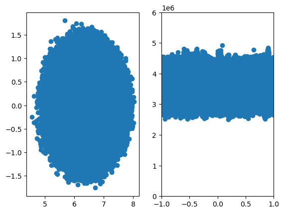
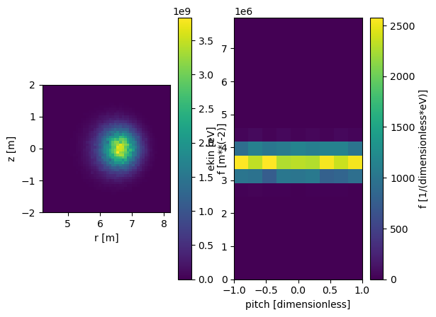
The generator works also when the momentum distribution is in \((E,\xi)\) basis. It also calculates the distribution of generated markers (with and without weights) so that these can be compared to the inputs.
[8]:
# Repeat the above example but with Exi distribution
alphadist = a5.data.active.getdist(
    "prod1", exi=True, ekin_edges=20, pitch_edges=10)
alphadist.integrate(time=np.s_[:], charge=np.s_[:])

# Generate markers
nmrk   = 10**6
anum   = 4
znum   = 2
mass   = 4.014*unyt.amu
charge = 2.0*unyt.e
mrk, mrkdist, prtdist = a5.markergen.generate(
    nmrk, mass, charge, anum, znum, alphadist, return_dists=True)

# Plot
mrkdist_rz  = mrkdist.integrate(ekin=np.s_[:], pitch=np.s_[:], phi=np.s_[:], copy=True)
mrkdist_exi = mrkdist.integrate(r=np.s_[:], z=np.s_[:], phi=np.s_[:], copy=True)

fig = plt.figure()
ax1 = fig.add_subplot(1,2,1)
mrkdist_rz.plot(axes=ax1)

ax2 = fig.add_subplot(1,2,2)
mrkdist_exi.plot(axes=ax2)
plt.show()
However, the markers that are created this way have all (almost) equal weights, i.e. the markers themselves have the same distribution as the alpha particles that are born. This might be undesirable if for example one is interested in wall loads: most alphas are born in the core and thus simulating those is just a waste of CPU time since they are unlikely to contribute to the losses.
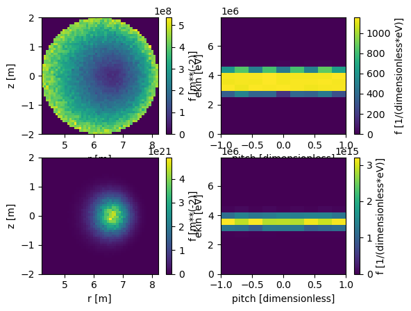
A better way is to have a separate distribution from which markers are sampled, and use the alpha particle birth distribution (or any other particle distribution) only to assign correct weights for the markers. To make a crude illustration of this idea, we define a marker distribution that is uniform in space, and reject markers whose weight is below some threshold. This way we get a distribution of markers that is uniform in space (inside the separatrix) and still represents the alpha particle population as a whole when weights (now non-identical) are included.
[9]:
# 5D (Exi) distribution of alphas
alphadist = a5.data.active.getdist(
    "prod1", exi=True, ekin_edges=20, pitch_edges=10)
alphadist.integrate(time=np.s_[:], charge=np.s_[:])

# Construct a 5D distribution that is uniform
markerdist = alphadist._copy()
markerdist._distribution[:] = 1

# Generate markers
nmrk   = 10**6
anum   = 4
znum   = 2
mass   = 4.014*unyt.amu
charge = 2.0*unyt.e
mrk, mrkdist, prtdist = a5.markergen.generate(
    nmrk, mass, charge, anum, znum, alphadist, markerdist=markerdist,
    return_dists=True, minweight=1)

# Plot both the distribution of markers and distribution of
# particles (markers with weights)
mrkdist_rz  = mrkdist.integrate(ekin=np.s_[:], pitch=np.s_[:], phi=np.s_[:], copy=True)
mrkdist_exi = mrkdist.integrate(r=np.s_[:], z=np.s_[:], phi=np.s_[:], copy=True)
prtdist_rz  = prtdist.integrate(ekin=np.s_[:], pitch=np.s_[:], phi=np.s_[:], copy=True)
prtdist_exi = prtdist.integrate(r=np.s_[:], z=np.s_[:], phi=np.s_[:], copy=True)

fig = plt.figure()
ax1 = fig.add_subplot(2,2,1)
mrkdist_rz.plot(axes=ax1)

ax2 = fig.add_subplot(2,2,3)
prtdist_rz.plot(axes=ax2)

ax3 = fig.add_subplot(2,2,2)
mrkdist_exi.plot(axes=ax3)

ax4 = fig.add_subplot(2,2,4)
prtdist_exi.plot(axes=ax4)
plt.show()
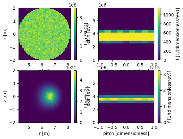
Specifying the marker distribution explicitly is not convenient, which is why there is a tool that converts a 1D profile to a 3D distribution. This still leaves one with the freedom to choose the momentum distribution as they wish. Here we use a rho profile that peaks towards the edge:
[10]:
# 5D (Exi) distribution of alphas
alphadist = a5.data.active.getdist(
    "prod1", exi=True, ekin_edges=20, pitch_edges=10)
alphadist.integrate(time=np.s_[:], charge=np.s_[:])

# Generate markerdist from a rho profile
rho  = np.linspace(0, 1, 100)
prob = np.ones((100,))
prob = (1.0+rho)**3

a5.input_init(bfield=True)
markerdist = a5.markergen.rhoto5d(
    rho, prob, alphadist.abscissa_edges("r"),
    alphadist.abscissa_edges("phi"), alphadist.abscissa_edges("z"),
    alphadist.abscissa_edges("ekin"), alphadist.abscissa_edges("pitch"))
a5.input_free()

# Generate markers
nmrk   = 10**6
anum   = 4
znum   = 2
mass   = 4.014*unyt.amu
charge = 2.0*unyt.e
mrk, mrkdist, prtdist = a5.markergen.generate(
    nmrk, mass, charge, anum, znum, alphadist, markerdist=markerdist,
    return_dists=True, minweight=1)

# Plot both the distribution of markers and distribution of
# particles (markers with weights)
mrkdist_rz  = mrkdist.integrate(ekin=np.s_[:], pitch=np.s_[:], phi=np.s_[:], copy=True)
mrkdist_exi = mrkdist.integrate(r=np.s_[:], z=np.s_[:], phi=np.s_[:], copy=True)
prtdist_rz  = prtdist.integrate(ekin=np.s_[:], pitch=np.s_[:], phi=np.s_[:], copy=True)
prtdist_exi = prtdist.integrate(r=np.s_[:], z=np.s_[:], phi=np.s_[:], copy=True)

fig = plt.figure()
ax1 = fig.add_subplot(2,2,1)
mrkdist_rz.plot(axes=ax1)

ax2 = fig.add_subplot(2,2,3)
prtdist_rz.plot(axes=ax2)

ax3 = fig.add_subplot(2,2,2)
mrkdist_exi.plot(axes=ax3)

ax4 = fig.add_subplot(2,2,4)
prtdist_exi.plot(axes=ax4)
plt.show()
AFSI5
Tag 6290a22
Branch docs

Note: Output file /home/runner/work/ascot5/ascot5/doc/tutorials/ascot.h5 is already present.

The qid of this run is 1845479973

Done