Finding orbit resonances and evaluating orbit-averaged quantities
In this tutorial, we will examine how the orbit diagnostics can be used to locate resonances and to evaluate orbit-averaged quantities.
We begin by initializing the standard test case. Note that the field has to be axisymmetric in order to gain meaningful results.
[1]:
import numpy as np
import unyt
import matplotlib.pyplot as plt
from a5py import Ascot

a5 = Ascot("ascot.h5", create=True)

a5.data.create_input("bfield analytical iter circular")
a5.data.create_input("wall_2D")
a5.data.create_input("plasma_1D")
a5.data.create_input("E_TC")
a5.data.create_input("N0_1D")
a5.data.create_input("asigma_loc")
a5.data.create_input("Boozer")
a5.data.create_input("MHD_STAT")

print("Inputs created")
/home/runner/work/ascot5/ascot5/a5py/routines/plotting.py:35: UserWarning: Could not import cKDTree and alphashape. 3D surface plotting disabled.
  warnings.warn(
Inputs created
Finding orbit resonances
A particle is in a resonance with a magnetic perturbation when the following condition is met:
where \(p\in\{\dots,-1,0,1,\dots\}\), \(\omega\) is the mode frequency (zero for static perturbations), \(n\) the poloidal mode number, and \(\omega_\mathrm{tor}\) and \(\omega_\mathrm{pol}\) are the (fast) particle toroidal and poloidal transit frequencies, respectively.
Orbit resonances are found by first populating the phase-space with markers of given species and then tracing those for several poloidal (and toroidal) orbits without collisions.
There are templates readily available that can be used to generate suitable marker population and simulation options. This example creates 10 (radial) \(\times\) 20 (pitch) alpha particles with \(E\) = 3.5 MeV that cover the radial grid from 0.3 to 1.0 and pitch from -1 to 1. The markers are simulated until they have either completed 12 toroidal or 6 poloidal transits.
NOTE: One full revolution around the poloidal (or toroidal) angle is considered to be a single poloidal (toroidal) transit. Since trapped particles don’t complete a full poloidal rotation, for those a single poloidal transit begins when the marker bounces for the first time, and ends with the third bounce (when it has returned to its original banana tip point, not in the position where it was launched).
[2]:
a5.input_init(bfield=True)
mrk = a5.data.create_input("marker resonance", species="alpha", rhogrid=np.linspace(0.3, 1.0, 10),
                           xigrid=np.linspace(-1, 1, 20), egrid=np.array([3.5e6])*unyt.eV, dryrun=True)
opt = a5.data.create_input("options singleorbit", ntor=12, npol=6, dryrun=True)
a5.input_free()
One can then run the simulation and post-process the results to find the orbit resonances.
However, there is also a method that: initializes the markers and the options, runs the simulation, and post-processes the results. You only have to specify the grids and the marker species (and initialize other input data).
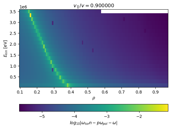
[3]:
rho = np.linspace(0.1, 0.97, 100)
xi  = 0.9
energy = np.linspace(0.1, 3.5, 20) * 1e6

a5.simulation_initinputs()
a5.input_eval_orbitresonance(rho, xi, energy, "alpha", plot=True, n=4, p=7, omega=0.0)
a5.simulation_free()
/usr/share/miniconda/envs/ascot-dev/lib/python3.10/site-packages/numpy/_core/fromnumeric.py:3858: RuntimeWarning: Mean of empty slice.
  return mean(axis=axis, dtype=dtype, out=out, **kwargs)
/usr/share/miniconda/envs/ascot-dev/lib/python3.10/site-packages/unyt/array.py:1972: RuntimeWarning: invalid value encountered in divide
  out_arr = func(
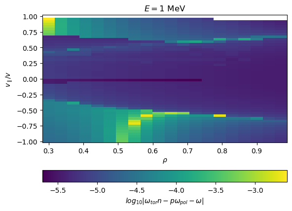
The resonance can be visualized also in (rho, pitch) and (pitch, energy) bases.
NOTE: This function performs poorly close to the magnetic axis as the current machinery doesn’t separate potato orbits.
[4]:
a5.simulation_initinputs()
rho = np.linspace(0.3, 0.97, 20)
xi = np.linspace(-1.0, 1.0, 50)
energy = 1.0e6
a5.input_eval_orbitresonance(rho, xi, energy, "alpha", plot=True, n=4, p=7, omega=0.0)
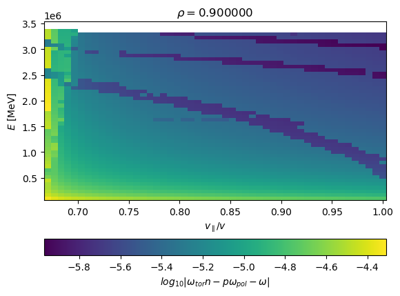
rho = 0.9
xi = np.linspace(0.67, 1.0, 50)
energy = np.linspace(0.1, 3.5) * 1e6
a5.input_eval_orbitresonance(rho, xi, energy, "alpha", plot=True, n=4, p=7, omega=0.0)
a5.simulation_free()
Evaluating orbit-averaged quantities
Orbit-averaged quantity is a mean value evaluated along the orbit trajectory:
where \(x\) is the quantity to be averaged along the orbit trajectory \((r(t), z(t))\), and \(\tau\) is the poloidal transit time.
This time we use templates and suitable options to trace a marker for a single poloidal orbit from which the orbit-averaged quantity can be calculated.
[5]:
a5.input_init(bfield=True)
mrk = a5.data.create_input("marker resonance", species="alpha", rhogrid=np.array([0.9]),
                           xigrid=np.array([0.8]), egrid=np.array([3.5e6])*unyt.eV, dryrun=True)
opt = a5.data.create_input("options singleorbit", ntor=10, npol=1, mode='prt', dryrun=True)
a5.input_free()

# We modify the options template to collect several data points along the orbit
# Remember to check that NPOINT value is sufficient so that the full orbit is
# captured
opt.update({
    "ORBITWRITE_MODE":1,
    "ORBITWRITE_NPOINT":1000,
    "ORBITWRITE_INTERVAL":1e-7,
})
Run the simulation and visualize the orbit.
[6]:
a5.simulation_initinputs()
a5.simulation_initoptions(**opt)
a5.simulation_initmarkers(**mrk)
vrun = a5.simulation_run(printsummary=False)

vrun.plotorbit_trajectory('r', 'z')
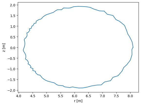
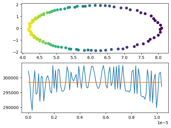
Now we can use these results to calculate the orbit averages.
[7]:
bphi, mu = vrun.getorbit('bphi', 'mu')
t, r, z, bphi, avg = vrun.getorbit_average(bphi, ids=1)
t, r, z,   mu, avg = vrun.getorbit_average(mu, ids=1)

fig = plt.figure()
ax1 = fig.add_subplot(2,1,1)
ax2 = fig.add_subplot(2,1,2)

print(r.shape,bphi.shape)
ax1.scatter(r, z, c=bphi, cmap='viridis')

ax2.plot(t, mu)
ax2.plot(t[[0,-1]], [avg, avg])

plt.show()

a5.simulation_free()
(104,) (104,)