Visualizing orbits

This example shows how to collect and visualize marker orbits.

Detailed description of the orbit collection options

The orbit data collection is one of the diagnostics that can be active in any simulation. Simply put, it records the marker position in phase-space (and some other quantities) at fixed time intervals or when a marker crosses a specific surface. The latter is used to generate Poincaré plots, while the former can be used to evaluate orbit-averaged quantities or just to visualize orbits. In simulations with large number of markers \((\gtrsim 10^4)\) the orbit data is rarely collected because it may use up a lot of memory and disk space.

The orbit data collection is enabled in options by setting ENABLE_ORBITWRITE = 1. The next option, ORBITWRITE_MODE, selects whether the marker trajectory is recorded when i) a given amount of time has passed or ii) marker crosses a predetermined surface. The latter is used for Poincaré plots, so choose ORBITWRITE_MODE=1 to collect the data in time intervals. The time interval is set by ORBITWRITE_INTERVAL which, if set to zero, collects the data at each integration time-step.

NOTE: The data is not collected exactly at ORBITWRITE_INTERVAL intervals, but on the first time step when at least the set amount of time has passed from the last time orbit data was recorded. If desired, the only way to collect the data at fixed intervals is to use a fixed time-step and choose ORBITWRITE_INTERVAL so that it is a multiple of the time-step.

Next we have ORBITWRITE_NPOINT which sets a maximum number of points kept in record for each marker. Roughly speaking, there is a fixed-size array in simulation for each marker that has length equal to this value, which is then filled one slot at a time every time the marker position is recorded. If this array becomes full, then the earliest record is overwritten, i.e, the array contains last ORBITWRITE_NPOINT records. If the array is not full at the end of the marker’s simulation, the unused slots are pruned before the data is written to disk.

Preferably ORBITWRITE_NPOINT is equal to the simulation time divided by ORBITWRITE_INTERVAL as then all the recorded points are kept. One can of course choose to keep only the last \(N\) values, which could be useful for debugging simulations or seeing how exactly markers ended up on the wall. Just keep in mind to not use a large value for ORBITWRITE_NPOINT in simulations with a large number of markers as that will easily eat all available RAM. It is a good practice to check how much data was allocated for the diagnostics when using the orbit collection. This value is printed at the beginning of the simulation after all inputs have been initialized.

Running a simulation where orbit data is being collected

First, initialize a test case where markers can be traced:

import numpy as np
from a5py import Ascot

a5 = Ascot("ascot.h5", create=True)
a5.data.create_input("bfield analytical iter circular")
a5.data.create_input("wall rectangular")
a5.data.create_input("plasma_1D")
a5.data.create_input("E_TC")
a5.data.create_input("N0_1D")
a5.data.create_input("Boozer")
a5.data.create_input("MHD_STAT")
a5.data.create_input("asigma_loc")

print("Inputs created")

Inputs created

As for markers, we create two alpha particles, one of which will not be confined in the simulation (for demonstration purposes):

from a5py.ascot5io.marker import Marker
mrk = Marker.generate("gc", n=2, species="alpha")
mrk["energy"][:] = 3.5e6

# Passing particle in the core = confined
mrk["ids"][0]   = 1
mrk["pitch"][0] = 0.9
mrk["r"][0]     = 7.2

# Banana on outward excursion near the edge = unconfined
mrk["ids"][1]   = 404
mrk["pitch"][1] = 0.5
mrk["r"][1]     = 8.1

a5.data.create_input("gc", **mrk)

'gc_2278882872'

Now we create options where the orbit data collection is enabled, and the data is collected at each time-step. Since we only have two markers, we set ORBITWRITE_NPOINT large enough to hold all recorded values. As for the simulation, we trace markers in hybrid mode (again for demonstration purposes) and enable orbit-following and set maximum mileage and wall collisions as end conditions.

from a5py.ascot5io.options import Opt

opt = Opt.get_default()
opt.update({
    # Settings specific for this tutorial
    "SIM_MODE":3, "ENABLE_ADAPTIVE":1,
    "ENDCOND_SIMTIMELIM":1, "ENDCOND_MAX_MILEAGE":1e-5,
    "ENDCOND_WALLHIT":1, "ENDCOND_MAX_RHO":1.0,
    "ENABLE_ORBIT_FOLLOWING":1,
    # Orbit diagnostics
    "ENABLE_ORBITWRITE":1, "ORBITWRITE_MODE":1,
    "ORBITWRITE_INTERVAL":0.0, "ORBITWRITE_NPOINT":10**4,
})
a5.data.create_input("opt", **opt, desc="HYBRID")

'opt_2365113065'

Now run the simulation:

import subprocess
subprocess.run(["./../../build/ascot5_main"])
print("Simulation completed")

ASCOT5_MAIN
Tag cc4ce10
Branch docs

Initialized MPI, rank 0, size 1.

Reading and initializing input.

Input file is ascot.h5.

Reading options input.
Active QID is 2365113065
Options read and initialized.

Reading magnetic field input.
Active QID is 4012828404

Analytical tokamak magnetic field (B_GS)
Psi at magnetic axis (6.618 m, -0.000 m)
-5.410 (evaluated)
-5.410 (given)
Magnetic field on axis:
B_R = 0.000 B_phi = 4.965 B_z = -0.000
Number of toroidal field coils 0
Estimated memory usage 0.0 MB
Magnetic field read and initialized.

Reading electric field input.
Active QID is 0729147563

Trivial Cartesian electric field (E_TC)
E_x = 0.000000e+00, E_y = 0.000000e+00, E_z = 0.000000e+00
Estimated memory usage 0.0 MB
Electric field read and initialized.

Reading plasma input.
Active QID is 3497298630

1D plasma profiles (P_1D)
Min rho = 0.00e+00, Max rho = 1.00e+02, Number of rho grid points = 3, Number of ion species = 1
Species Z/A  charge [e]/mass [amu] Density [m^-3] at Min/Max rho    Temperature [eV] at Min/Max rho
   1  /  1     1  /  1.000             1.00e+20/1.00e+20                1.00e+20/1.00e+20
[electrons]   -1  /  0.001             1.00e+20/1.00e+20                1.00e+03/1.00e+03
Quasi-neutrality is (electron / ion charge density) 1.00
Estimated memory usage 0.0 MB
Plasma data read and initialized.

Reading neutral input.
Active QID is 0252834829

1D neutral density and temperature (N0_1D)
Grid:  nrho =    3   rhomin = 0.000   rhomax = 2.000
 Number of neutral species = 1
Species Z/A   (Maxwellian)
        1/  1 (1)
Estimated memory usage 0.0 MB
Neutral data read and initialized.

Reading wall input.
Active QID is 0765367556

2D wall model (wall_2D)
Number of wall elements = 20, R extend = [4.10, 8.40], z extend = [-3.90, 3.90]
Estimated memory usage 0.0 MB
Wall data read and initialized.

Reading boozer input.
Active QID is 1417268624

Boozer input
psi grid: n =    6 min = 0.000 max = 1.000
thetageo grid: n =   18
thetabzr grid: n =   10
Boozer data read and initialized.

Reading MHD input.
Active QID is 3942259169

MHD (stationary) input
Grid: nrho =    6 rhomin = 0.000 rhomax = 1.000

Modes:
(n,m) = ( 1, 3) Amplitude = 0.1 Frequency =   1 Phase =   0
(n,m) = ( 2, 4) Amplitude =   2 Frequency = 1.5 Phase = 0.785
Estimated memory usage 0.0 MB
MHD data read and initialized.

Reading atomic reaction input.
Active QID is 0541688633

Found data for 1 atomic reactions:
Reaction number / Total number of reactions = 1 / 1
  Reactant species Z_1 / A_1, Z_2 / A_2     = 1 / 1, 1 / 1
  Min/Max energy                            = 1.00e+03 / 1.00e+04
  Min/Max density                           = 1.00e+18 / 1.00e+20
  Min/Max temperature                       = 1.00e+03 / 1.00e+04
  Number of energy grid points              = 3
  Number of density grid points             = 4
  Number of temperature grid points         = 5
Estimated memory usage 0.0 MB
Atomic reaction data read and initialized.

Reading marker input.
Active QID is 2278882872

Loaded 2 guiding centers.
Marker data read and initialized.

All input read and initialized.

Initializing marker states.
Estimated memory usage 0.0 MB.
Marker states initialized.
Initialized diagnostics, 2.9 MB.

Preparing output.
Note: Output file ascot.h5 is already present.

The qid of this run is 1098871079

Inistate written.
Simulation begins; 4 threads.
Simulation complete.
Simulation finished in 0.013610 s
Endstate written.

Combining and writing diagnostics.

Writing diagnostics output.
Writing orbit diagnostics.

Diagnostics output written.
Diagnostics written.

Summary of results:
        1 markers had end condition Sim time limit
        1 markers had end condition Wall collision

          No markers were aborted.

Done.
Simulation completed

The orbit data is accessed by using the run group’s getorbit method:

a5 = Ascot("ascot.h5")

# Retrieve mileage
mil = a5.data.active.getorbit("ekin")

# Multiple quantities can be accessed simultaneously
# (which is more efficient than accessing individually)
r, z = a5.data.active.getorbit("r", "z")

# Data can be parsed by marker ID
rho = a5.data.active.getorbit("rho", ids=1)
rho = a5.data.active.getorbit("rho", ids=[1,404])

# ...or by end condition
rho = a5.data.active.getorbit("rho", endcond="NOT WALL")
rho = a5.data.active.getorbit("rho", endcond=["TLIM", "WALL"])

Some quantities are evaluated run-time and some of those requires access to input data, or otherwise exception is raised:

a5.input_init(bfield=True)
psi = a5.data.active.getorbit("psi", ids=404)
a5.input_free(bfield=True)

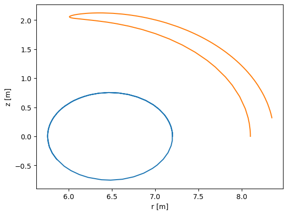
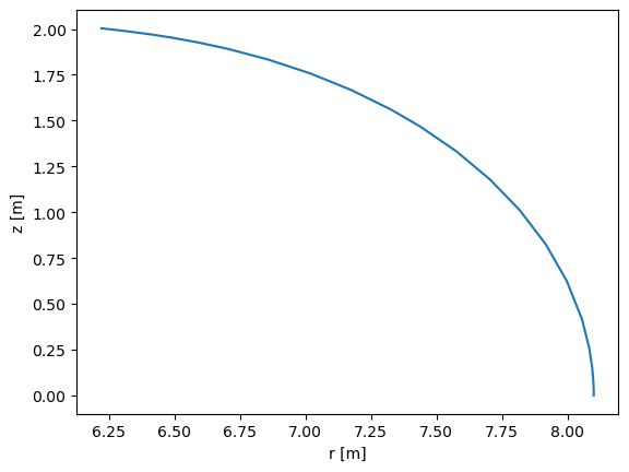
Orbits can also be plotted easily with the plotorbit_trajectory method:

a5.data.active.plotorbit_trajectory("r", "z", endcond="TLIM")
a5.data.active.plotorbit_trajectory("mileage", "ekin", ids=404)

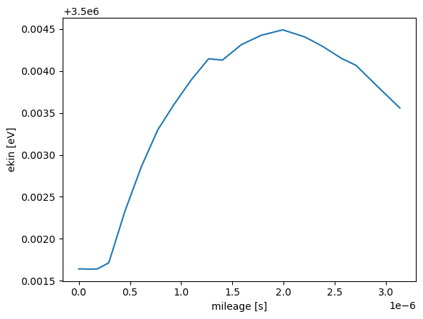
With the orbit data it is not possible to choose if the quantities are evaluated in particle or guiding-center coordinates with the reason being that only one these are stored. So which one?

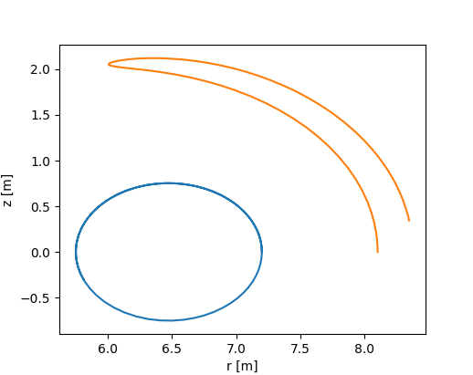
By default, the one corresponding to the simulation mode: particle coordinates in GO simulation and guiding-center coordinates in GC simulation. In hybrid mode, the stored quantity corresponds to simulation mode that was active at the moment. This is why there is a “jump” of 500 eV in energy in the plot above, which corresponds to time instant when the simulation changed from guiding center to hybrid. This is more clearly visible if we plot the orbit poloidal trajectory:

a5.data.active.plotorbit_trajectory("r", "z", ids=404)

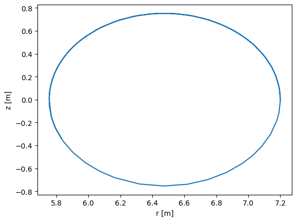
It is possible to force the code to collect only the guiding center data (even in GO mode):

opt = a5.data.options.active.read()
opt.update({"RECORD_MODE":1})

a5.simulation_initinputs()
a5.simulation_initoptions(**opt)

mrk = a5.data.marker.active.read()
a5.simulation_initmarkers(**mrk)

vrun = a5.simulation_run(printsummary=False)

vrun.plotorbit_trajectory("r", "z")
a5.simulation_free()

/home/runner/work/ascot5/ascot5/a5py/ascotpy/libsimulate.py:297: AscotUnitWarning: Argument(s) r, phi, z, time, mass, charge, energy, zeta given without dimensions (assumed m, degree, m, s, amu, e, eV, rad)
  r, phi, z, t, m, q, energy, pitch, zeta, anum, znum, w, ids = parse(