Estimating wall loads
This example shows how to estimate and visualize wall loads.
Accurate modelling of the wall loads is one of the most computationally expensive operations one can use ASCOT5 for because it can require millions of markers. Therefore it is worthwhile to invest in marker generation and pre-selection, but those topics are discussed in a separate example.
In this example we focus just on the wall loads. Therefore we generate neutral markers which obviously are lost instantly.
[1]:
import numpy as np
import unyt
import matplotlib.pyplot as plt
from a5py import Ascot

a5 = Ascot("ascot.h5", create=True)

a5.data.create_input("bfield analytical iter circular")
a5.data.create_input("plasma flat")
a5.data.create_input("E_TC")
a5.data.create_input("N0_1D")
a5.data.create_input("Boozer")
a5.data.create_input("MHD_STAT")
a5.data.create_input("asigma_loc")

# Neutrals with a random velocity vector
power = 1.0e7 * unyt.W
from a5py.ascot5io.marker import Marker
nmrk = 10**5
mrk = Marker.generate("gc", n=nmrk, species="alpha")
mrk["charge"][:] = 0
mrk["energy"][:] = 3.5e6
mrk["pitch"][:]  = 0.999 - 1.998 * np.random.rand(nmrk,)
mrk["zeta"][:]   = 2*np.pi * np.random.rand(nmrk,)
mrk["r"][:]      = 8.5
mrk["z"][:]      = 0.0
mrk["phi"][:]    = 180
mrk["weight"][:] = (power / (nmrk * mrk["energy"])).to("particles/s")
a5.data.create_input("gc", **mrk)

print("Inputs created")
/home/runner/work/ascot5/ascot5/a5py/routines/plotting.py:35: UserWarning: Could not import cKDTree and alphashape. 3D surface plotting disabled.
  warnings.warn(
Inputs created
The other relevant input is the 3D wall as the wall loads can’t be estimated with a 2D wall (whose linear elements have no area!). Experience has shown that while the magnetic field perturbations governs how much and where particles are lost, the wall shape has a huge impact on the values of the wall loads and where exactly the hot spots form. Hence an accurate wall geometry is essential for accurate results.
But since we are simulating neutral particles born on-axis and immune to ionization, we clearly don’t care about accuracy and our 3D wall is just a 2D contour that is revolved toroidally:
[2]:
from a5py.ascot5io.wall import wall_3D

rad  = 2.0
pol  = np.linspace(0, 2*np.pi, 181)[:-1]
w2d = {"nelements":180,
       "r":7.0 + rad*np.cos(pol), "z":rad*np.sin(pol)}
w3d = wall_3D.convert_wall_2D(180, **w2d)
The origin of the wall mesh is usually a CAD model where different regions of the wall are clearly defined. In ASCOT5, those are all clumped together into a single triangular mesh. However, different regions of the wall can be separated by marking the corresponding triangles with flags. In this example, we divide the mesh into three regions: top, mid, and bottom, based on the triangle z-coordinate.
[3]:
idtop = w3d["z1z2z3"][:,0] > 1
idmid = np.logical_and(w3d["z1z2z3"][:,0] <= 1, w3d["z1z2z3"][:,0] >= -1)
idbottom = w3d["z1z2z3"][:,0] < -1

labels = {"top":1, "mid":2, "bottom":3}

w3d["flag"] = np.zeros((w3d["nelements"],1))
w3d["labels"] = labels
w3d["flag"][idtop] = labels["top"]
w3d["flag"][idmid] = labels["mid"]
w3d["flag"][idbottom] = labels["bottom"]
a5.data.create_input("wall_3D", **w3d, desc="REVOLVED")
[3]:
'wall_3D_0386375317'
While engineers weep, we set up the simulation options and run the code. In options the only noteworthy parameters are that the wall hit end condition is enabled, and that we use gyro-orbit simulation mode. Guiding-center simulations also produce wall hits but they might underestimate the loads or hit “wrong” spots if the Larmor radius is large.
[4]:
from a5py.ascot5io.options import Opt

opt = Opt.get_default()
opt.update({
    # Simulation mode
    "SIM_MODE":1, "FIXEDSTEP_USE_USERDEFINED":1, "FIXEDSTEP_USERDEFINED":1e-8,
    # Setting max mileage above slowing-down time is a good safeguard to ensure
    # simulation finishes even with faulty inputs. Same with the CPU time limit.
    "ENDCOND_WALLHIT":1,
    # Physics
    "ENABLE_ORBIT_FOLLOWING":1,
})
a5.data.create_input("opt", **opt, desc="WALLHITS")
[4]:
'opt_4136037998'
[5]:
import subprocess
subprocess.run(["./../../build/ascot5_main", "--d=\"GREATESTHITS\""])
print("Simulation completed")
ASCOT5_MAIN
Tag 6290a22
Branch docs

Initialized MPI, rank 0, size 1.

Reading and initializing input.

Input file is ascot.h5.

Reading options input.
Active QID is 4136037998
Options read and initialized.

Reading magnetic field input.
Active QID is 3156855207

Analytical tokamak magnetic field (B_GS)
Psi at magnetic axis (6.618 m, -0.000 m)
-5.410 (evaluated)
-5.410 (given)
Magnetic field on axis:
B_R = 0.000 B_phi = 4.965 B_z = -0.000
Number of toroidal field coils 0
Magnetic field read and initialized.

Reading electric field input.
Active QID is 3096286506

Trivial Cartesian electric field (E_TC)
E_x = 0.000000e+00, E_y = 0.000000e+00, E_z = 0.000000e+00
Electric field read and initialized.

Reading plasma input.
Active QID is 0339773264

1D plasma profiles (P_1D)
Min rho = 0.00e+00, Max rho = 1.00e+01, Number of rho grid points = 100, Number of ion species = 1
Species Z/A  charge [e]/mass [amu] Density [m^-3] at Min/Max rho    Temperature [eV] at Min/Max rho
   1  /  1     1  /  1.000             1.00e+21/1.00e+00                1.00e+04/1.00e+04
[electrons]   -1  /  0.001             1.00e+21/1.00e+00                1.00e+04/1.00e+04
Toroidal rotation [rad/s] at Min/Max rho: 0.00e+00/0.00e+00
Quasi-neutrality is (electron / ion charge density) 1.00
Toroidal rotation [rad/s] at Min/Max rho: 0.00e+00/0.00e+00
Plasma data read and initialized.

Reading neutral input.
Active QID is 1454727964

1D neutral density and temperature (N0_1D)
Grid:  nrho =    3   rhomin = 0.000   rhomax = 2.000
 Number of neutral species = 1
Species Z/A   (Maxwellian)
        1/  1 (1)
Neutral data read and initialized.

Reading wall input.
Active QID is 0386375317

3D wall model (wall_3D)
Number of wall elements 64800
Spanning xmin = -9.100 m, xmax = 9.100 m
         ymin = -9.100 m, ymax = 9.100 m
         zmin = -2.100 m, zmax = 2.100 m
Wall data read and initialized.

Reading boozer input.
Active QID is 0293741184

Boozer input
psi grid: n =    6 min = 0.000 max = 1.000
thetageo grid: n =   18
thetabzr grid: n =   10
Boozer data read and initialized.

Reading MHD input.
Active QID is 1588733380

MHD (stationary) input
Grid: nrho =    6 rhomin = 0.000 rhomax = 1.000

Modes:
(n,m) = ( 1, 3) Amplitude = 0.1 Frequency =   1 Phase =   0
(n,m) = ( 2, 4) Amplitude =   2 Frequency = 1.5 Phase = 0.785
MHD data read and initialized.

Reading atomic reaction input.
Active QID is 1847566086

Found data for 1 atomic reactions:
Reaction number / Total number of reactions = 1 / 1
  Reactant species Z_1 / A_1, Z_2 / A_2     = 0 / 0, 0 / 0
  Min/Max energy                            = 1.00e+03 / 1.00e+04
  Min/Max density                           = 1.00e+18 / 1.00e+20
  Min/Max temperature                       = 1.00e+03 / 1.00e+04
  Number of energy grid points              = 3
  Number of density grid points             = 4
  Number of temperature grid points         = 5
Atomic reaction data read and initialized.

Reading marker input.
Active QID is 4263595949

Loaded 100000 guiding centers.
Marker data read and initialized.

All input read and initialized.

Initializing marker states.
Estimated memory usage 0.8 MB.
Marker states initialized.

Preparing output.
Note: Output file ascot.h5 is already present.

The qid of this run is 0865315969

Inistate written.
Simulation begins; 4 threads.
Simulation complete.
Simulation finished in 0.516404 s
Endstate written.

Combining and writing diagnostics.

Writing diagnostics output.

Diagnostics output written.
Diagnostics written.

Summary of results:
   100000 markers had end condition Wall collision

          No markers were aborted.

Done.
Simulation completed
Now to visualize wall loads. First we want to print the 0D quantities and then plot the wall load histogram. Note how the flags can be used to filter the results.
[6]:
a5 = Ascot("ascot.h5") # Refresh data

warea_total, peak_total = a5.data.active.getwall_figuresofmerit()
warea_top, peak_top = a5.data.active.getwall_figuresofmerit(flags=1)
warea_rest, peak_rest = a5.data.active.getwall_figuresofmerit(flags=["mid", "bottom"])
print(f"Wetted area: {warea_top} (top), {warea_rest} (rest), {warea_total} (total)")
print(
    f"Peak power load: {peak_top.to('MW/m**2')} (top), "
    f"{peak_rest.to('MW/m**2')} (rest), {peak_total.to('MW/m**2')} (total)"
    )

fig = plt.figure()
ax1 = fig.add_subplot(1,3,1)
a5.data.active.plotwall_loadvsarea(flags="top", axes=ax1)
ax1.set_title("Top")
ax2 = fig.add_subplot(1,3,2)
a5.data.active.plotwall_loadvsarea(flags="mid", axes=ax2)
ax2.set_title("Mid")
ax3 = fig.add_subplot(1,3,3)
a5.data.active.plotwall_loadvsarea(flags="bottom", axes=ax3)
ax3.set_title("Bottom")
plt.show()
Wetted area: 48.763116848093205 m**2 (top), 103.89137064283472 m**2 (rest), 152.65448749092792 m**2 (total)
Peak power load: 0.5474577100048088 MW/m**2 (top), 3.246660530293389 MW/m**2 (rest), 3.246660530293389 MW/m**2 (total)
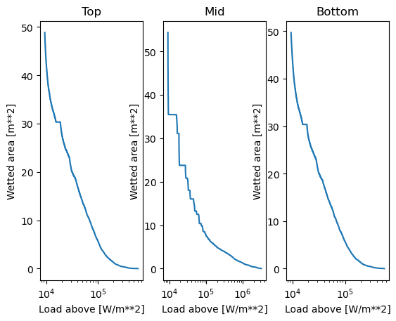
Note that the histogram shows the wetted area cumulatively; the value on the \(y\)-axis corresponds to the area where the load is at least the amount given by the \(x\)-axis.
Now where on the wall the particles ended and are there any hot-spots? This plot uses the magnetic axis to calculate the poloidal angle, which is why the magnetic field data has to be initialized.
[7]:
a5.input_init(bfield=True)
fig = plt.figure(figsize=(15,4))
ax1 = fig.add_subplot(1,2,1)
a5.data.active.plotwall_torpol(qnt="label", axes=ax1)
ax1.set_title("Label")
ax2 = fig.add_subplot(1,2,2)
a5.data.active.plotwall_torpol(qnt="eload", axes=ax2)
ax2.set_title("Power load")
a5.input_free()
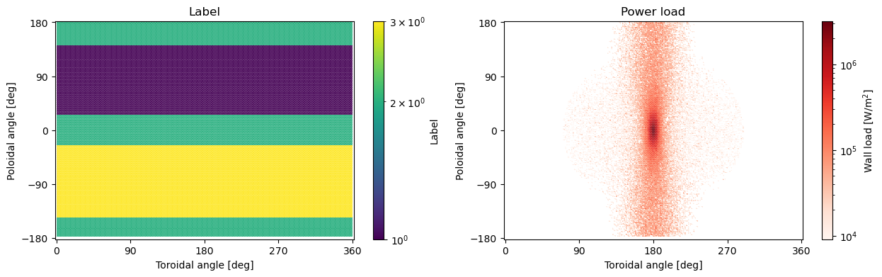
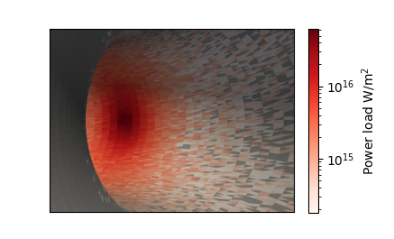
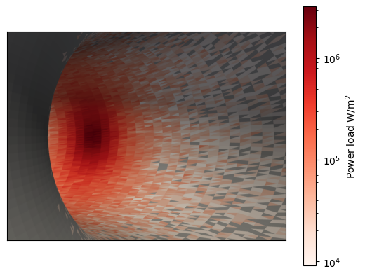
While previous plot is good for giving a sense of how the loads are distributed, it skews the areas. The way to properly visualize the wall loads is with a 3D plot. Plotting in 3D requires Visualization Toolkit (VTK) and this doesn’t work that well in Jupyter notebooks, which is why the command below might give a warning and the figure might appear twice (this issue only affects notebooks and not normal work with ASCOT5).
[8]:
a5.data.active.plotwall_3dstill(cpos=(0,6.9,0), cfoc=(0,7.0,0), cang=(120,0,-90), data="eload", log=True)
/home/runner/work/ascot5/ascot5/a5py/routines/plotting.py:1277: UserWarning: Failed to use notebook backend:

No module named 'trame'

Falling back to a static output.
  p.show()

You can also make an interactive plot with a5.data.active.plotwall_3dinteractive(). The most convenient way to investigate a 3D plot is to use a5gui where one can record the camera position in an interactive plot, and use it in stills.
The 3D plotting tools in ASCOT5 are rudimentary, since there are dedicated external tools for visualizing 3D meshes. The wall data including the wall loads can be saved to disk in a desired format (e.g. vtk, stl):
[9]:
mesh = a5.data.active.getwall_3dmesh()

# Shows what fields are in the cell data
mesh.cell_data

# To save the data as a vtk file, use mesh.save("mesh.vtk")
[9]:
pyvista DataSetAttributes
Association     : CELL
Active Scalars  : label
Active Vectors  : None
Active Texture  : None
Active Normals  : None
Contains arrays :
    label                   int32      (64800,)             SCALARS
    pload                   float64    (64800,)
    eload                   float64    (64800,)
    mload                   float64    (64800,)
    iangle                  float64    (64800,)