Introduction

This example gives a general overview on how to pre- and postprocess ASCOT5 simulations.

1. First simulation: step-by-step

2. Contents of the HDF5 file

3. Python interface to libascot.so

4. Input generation

5. Post processing

6. Live simulations

First simulation: step-by-step

Go to ascot5/doc/tutorials folder and type ipython3 to begin this tutorial. Then repeat these steps:

1. All pre- and post-processing is done via Ascot object. To create a new ASCOT5 data file, use create=True.

import numpy as np
from a5py import Ascot

a5 = Ascot("ascot.h5", create=True)
print("File created")

File created

2. The following lines initialize test data. We will go through the input generation in detail later.

# Use pre-existing template to create some input data
a5.data.create_input("options tutorial")
a5.data.create_input("bfield analytical iter circular")
a5.data.create_input("wall rectangular")
a5.data.create_input("plasma flat")

# Create electric field and markers by giving input parameters explicitly
from a5py.ascot5io.marker import Marker
mrk = Marker.generate("gc", n=100, species="alpha")
mrk["energy"][:] = 3.5e6
mrk["pitch"][:]  = 0.99 - 1.98 * np.random.rand(100,)
mrk["r"][:]      = np.linspace(6.2, 8.2, 100)
a5.data.create_input("gc", **mrk)
a5.data.create_input("E_TC", exyz=np.array([0,0,0])) # Zero electric field

# Create dummy input for the rest
a5.data.create_input("N0_3D")
a5.data.create_input("Boozer")
a5.data.create_input("MHD_STAT")
a5.data.create_input("asigma_loc")
print("Inputs initialized")

Inputs initialized

/home/runner/work/ascot5/ascot5/a5py/ascot5io/__init__.py:242: AscotUnitWarning: Argument(s) weight given without dimensions (assumed 1/s)
  name = HDF5TOOBJ[inp].write_hdf5(

3. EITHER close the ipython session and edit options on terminal (opens a text editor):

   a5editoptions ascot.h5

   Scroll down to “End conditions” and set ENDCOND_MAX_MILEAGE = 0.5e-2. Save and close the editor. When prompted, set “Fast” as a description.

   OR set the options in ipython:

name = a5.data.options.active.new(ENDCOND_MAX_MILEAGE=0.5e-2, desc="Fast")
a5.data.options[name].activate()
print("Options updated")

Options updated

4. Now execute ascot5_main which should take less than 10 seconds.

   EITHER in terminal:

   ./../../build/ascot5_main --d="Hello world!"

   OR in ipython:

import subprocess
subprocess.run(["./../../build/ascot5_main", "--d=\"Hello world!\""])
print("Simulation completed")

ASCOT5_MAIN
Tag 20656e3
Branch docs

Initialized MPI, rank 0, size 1.

Reading and initializing input.

Input file is ascot.h5.

Reading options input.
Active QID is 2898783227
Options read and initialized.

Reading magnetic field input.
Active QID is 3610091528

Analytical tokamak magnetic field (B_GS)
Psi at magnetic axis (6.618 m, -0.000 m)
-5.410 (evaluated)
-5.410 (given)
Magnetic field on axis:
B_R = 0.000 B_phi = 4.965 B_z = -0.000
Number of toroidal field coils 0
Estimated memory usage 0.0 MB
Magnetic field read and initialized.

Reading electric field input.
Active QID is 2624549030

Trivial Cartesian electric field (E_TC)
E_x = 0.000000e+00, E_y = 0.000000e+00, E_z = 0.000000e+00
Estimated memory usage 0.0 MB
Electric field read and initialized.

Reading plasma input.
Active QID is 0477821367

1D plasma profiles (P_1D)
Min rho = 0.00e+00, Max rho = 1.00e+01, Number of rho grid points = 100, Number of ion species = 1
Species Z/A  charge [e]/mass [amu] Density [m^-3] at Min/Max rho    Temperature [eV] at Min/Max rho
   1  /  1     1  /  1.000             1.00e+21/1.00e+00                1.00e+04/1.00e+04
[electrons]   -1  /  0.001             1.00e+21/1.00e+00                1.00e+04/1.00e+04
Quasi-neutrality is (electron / ion charge density) 1.00
Estimated memory usage 0.0 MB
Plasma data read and initialized.

Reading neutral input.
Active QID is 3090815515

3D neutral density and temperature (N0_3D)
Grid:  nR =    3   Rmin = 0.000   Rmax = 100.000
       nz =    3   zmin = -100.000   zmax = 100.000
     nphi =    3 phimin = 0.000 phimax = 6.283
 Number of neutral species = 1
Species Z/A   (Maxwellian)
        1/  1 (1)
Estimated memory usage 0.0 MB
Neutral data read and initialized.

Reading wall input.
Active QID is 0593796151

2D wall model (wall_2D)
Number of wall elements = 20, R extend = [4.10, 8.40], z extend = [-3.90, 3.90]
Estimated memory usage 0.0 MB
Wall data read and initialized.

Reading boozer input.
Active QID is 1989571515

Boozer input
psi grid: n =    6 min = 0.000 max = 1.000
thetageo grid: n =   18
thetabzr grid: n =   10
Boozer data read and initialized.

Reading MHD input.
Active QID is 1637756274

MHD (stationary) input
Grid: nrho =    6 rhomin = 0.000 rhomax = 1.000

Modes:
(n,m) = ( 1, 3) Amplitude = 0.1 Frequency =   1 Phase =   0
(n,m) = ( 2, 4) Amplitude =   2 Frequency = 1.5 Phase = 0.785
Estimated memory usage 0.0 MB
MHD data read and initialized.

Reading atomic reaction input.
Active QID is 1074986078

Found data for 1 atomic reactions:
Reaction number / Total number of reactions = 1 / 1
  Reactant species Z_1 / A_1, Z_2 / A_2     = 1 / 1, 1 / 1
  Min/Max energy                            = 1.00e+03 / 1.00e+04
  Min/Max density                           = 1.00e+18 / 1.00e+20
  Min/Max temperature                       = 1.00e+03 / 1.00e+04
  Number of energy grid points              = 3
  Number of density grid points             = 4
  Number of temperature grid points         = 5
Estimated memory usage 0.0 MB
Atomic reaction data read and initialized.

Reading marker input.
Active QID is 3700504171

Loaded 100 guiding centers.
Marker data read and initialized.

All input read and initialized.

Initializing marker states.
Estimated memory usage 0.0 MB.
Marker states initialized.

Preparing output.
Note: Output file ascot.h5 is already present.

The qid of this run is 1534853437

Inistate written.
Initialized diagnostics, 536.0 MB.
host: All fields initialized. Simulation begins, 4 threads.
host: Simulation complete.
process 0 finished: gpu 0.000000 s, host 2.602025 s
Endstate written.

Combining and writing diagnostics.

Writing diagnostics output.

Writing 5D distribution.

Writing 6D distribution.

Writing rho 5D distribution.

Writing rho 6D distribution.

Writing COM distribution.
Writing orbit diagnostics.

Diagnostics output written.
Diagnostics written.

Summary of results:
       98 markers had end condition Sim time limit
        2 markers had end condition Wall collision

          No markers were aborted.

Done.
Simulation completed

5. Open ipython again to read the data and plot marker endstates.

   Hint: You can add the line from a5py import Ascot to your ipython config file (~/.ipython/profile_default/ipython_config.py) so that it is automatically called in beginning of every ipython session:

        c = get_config()
        c.InteractiveShellApp.exec_lines = [
            '%load_ext autoreload',
            '%autoreload 2',
            'import numpy as np',
            'import scipy',
            'import matplotlib as mpl',
            'import matplotlib.pyplot as plt',
            'from a5py import Ascot',
        ]
   

from a5py import Ascot
import numpy as np
import matplotlib.pyplot as plt

a5 = Ascot("ascot.h5")
a5.data.ls(show=True) # Print summary of the data within this file
mil = a5.data.active.getstate("mileage", state="end") # How much time passed for each marker
print("Average mileage: %0.5f" % (np.mean(mil)))

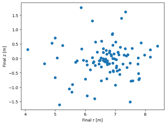
# Plots markers' final (R, z) coordinates and wall contour
ax = plt.figure().add_subplot(1,1,1)
a5.data.active.plotstate_scatter("end r", "end z", axes=ax)
plt.show(block=False)

Inputs: [only active shown]
options opt        2898783227 2024-05-06 07:00:42
Fast
+ 1 other(s)
bfield  B_GS       3610091528 2024-05-06 07:00:42
TAG
+ 0 other(s)
efield  E_TC       2624549030 2024-05-06 07:00:42
TAG
+ 0 other(s)
marker  gc         3700504171 2024-05-06 07:00:42
TAG
+ 0 other(s)
plasma  plasma_1D  0477821367 2024-05-06 07:00:42
TAG
+ 0 other(s)
neutral N0_3D      3090815515 2024-05-06 07:00:42
DUMMY
+ 0 other(s)
wall    wall_2D    0593796151 2024-05-06 07:00:42
TAG
+ 0 other(s)
boozer  Boozer     1989571515 2024-05-06 07:00:42
DUMMY
+ 0 other(s)
mhd     MHD_STAT   1637756274 2024-05-06 07:00:42
DUMMY
+ 0 other(s)
asigma  asigma_loc 1074986078 2024-05-06 07:00:42
DUMMY
+ 0 other(s)
Results:
run        1534853437 2024-05-06 07:00:42. [active]
"Hello world!"

Average mileage: 0.00490

6. That’s it! Now you have prepared inputs, ran ASCOT5, and accessed the simulation output.

   For actual simulations each step is more involving, but the basic premise was illustrated here. ASCOT5 development aims to integrate most input generation and post-processing tools so that they can be accessed via an Ascot object. Therefore, it is a good idea to always check from the documentation if there is an existing tool available.

   Next in this tutorial, we will go through each step in detail. However, don’t forget to try ASCOT5 GUI for fast and easy access to the data (type a5gui ascot.h5 in terminal to open it).

Contents of the HDF5 file

ASCOT5 stores the data in a HDF5 file. The file contains all inputs necessary to (re)run the simulation and the simulation output. The format supports multiple inputs and multiple outputs so that all data relevant for a single study can be stored in a single file (but remember to make backups!). To separate inputs and simulations from one another, each input and each simulation is assigned a quasi-unique identifier (QID) which is string of ten numbers from 0-10.

How exactly the data is stored in a file is not relevant, as the data is accessed via Ascot object. Or to be more precise, the contents of the file is accessed and modified via Ascot.data attribute which is an Ascot5IO object.

The contents of the file can be quickly viewed with ls() method (GUI is also very good for this purpose).

# In ipython terminal:
from a5py import Ascot
a5 = Ascot("ascot.h5")
info = a5.data.ls()

Inputs: [only active shown]
options opt        2898783227 2024-05-06 07:00:42
Fast
+ 1 other(s)
bfield  B_GS       3610091528 2024-05-06 07:00:42
TAG
+ 0 other(s)
efield  E_TC       2624549030 2024-05-06 07:00:42
TAG
+ 0 other(s)
marker  gc         3700504171 2024-05-06 07:00:42
TAG
+ 0 other(s)
plasma  plasma_1D  0477821367 2024-05-06 07:00:42
TAG
+ 0 other(s)
neutral N0_3D      3090815515 2024-05-06 07:00:42
DUMMY
+ 0 other(s)
wall    wall_2D    0593796151 2024-05-06 07:00:42
TAG
+ 0 other(s)
boozer  Boozer     1989571515 2024-05-06 07:00:42
DUMMY
+ 0 other(s)
mhd     MHD_STAT   1637756274 2024-05-06 07:00:42
DUMMY
+ 0 other(s)
asigma  asigma_loc 1074986078 2024-05-06 07:00:42
DUMMY
+ 0 other(s)
Results:
run        1534853437 2024-05-06 07:00:42. [active]
"Hello world!"

The data attribute provides a treeview of the contents. At the top level are input parent groups, e.g. bfield, and result groups. Each input parent group contains all inputs in that category, e.g. bfield contains every magnetic field input. The one that is going to be used in a simulation is marked with an active flag. Again, ls() method can be used to view the contents of input parent groups.

info = a5.data.options.ls()

opt        2898783227 2024-05-06 07:00:42 [active]
Fast
opt        2322963913 2024-05-06 07:00:42
TAG

As can be seen, each input has a QID (the quasi-unique identifier), date when it was created, user-given description, and name that has a format <inputtype>_<qid>. Note that when we used a5editoptions to modify options, the old options were preserved.

Objects representing the inputs can be accessed via their name, qid, or tag which is the first word in the description. Both attribute-like and dictionary-like referencing is supported.

# These all point to same object (note that this cell fails if commented lines are uncommented without using proper QID)
#a5.data.options.q1234567890       # Ref by QID, note "q" prefix
a5.data.options.FAST               # Ref by tag, note that it is always all caps, no special symbols allowed and max 10 characters
#a5.data.options.Opt_1234567890    # Ref by name
a5.data.options.active             # Ref to options input that is currently active and will be used in the next simulation
#a5.data["options"]["q1234567890"] # Dictionary-like access

<a5py.ascot5io.options.Opt at 0x7f275aa013c0>

Each input object (as well as result group) has methods to access its meta data and alter the description (and, hence, tag). The inbut objects don’t read the actual data when Ascot object is initialized to keep it light-weight. The read method reads the raw data from the HDF5 file but for post-processing purposes there are better tools which are introduced later.

a5.data.options.active.get_qid()
a5.data.options.active.get_date()
a5.data.options.active.get_name()

a5.data.options.active.set_desc("New tag")
# The tag was updated
a5.data.options.NEW.get_desc()
a5.data.options.active.activate() # Set group as active
#a5.data.options.active.destroy() # This would remove the data from the HDF5 file
a5.data.options.active.read()

{'ADAPTIVE_MAX_DPHI': 2.0,
 'ADAPTIVE_MAX_DRHO': 0.1,
 'ADAPTIVE_TOL_CCOL': 0.1,
 'ADAPTIVE_TOL_ORBIT': 1e-08,
 'DISABLE_ENERGY_CCOLL': 0,
 'DISABLE_FIRSTORDER_GCTRANS': 0,
 'DISABLE_GCDIFF_CCOLL': 0,
 'DISABLE_PITCH_CCOLL': 0,
 'DIST_MAX_CHARGE': 2.5,
 'DIST_MAX_EKIN': 1e-12,
 'DIST_MAX_MU': 2.5e-13,
 'DIST_MAX_PHI': 360.0,
 'DIST_MAX_PPA': 1e-19,
 'DIST_MAX_PPE': 1e-19,
 'DIST_MAX_PPHI': 1e-19,
 'DIST_MAX_PR': 1e-19,
 'DIST_MAX_PTOR': 1e-18,
 'DIST_MAX_PZ': 1e-19,
 'DIST_MAX_R': 8.5,
 'DIST_MAX_RHO': 1.0,
 'DIST_MAX_THETA': 360.0,
 'DIST_MAX_TIME': 0.03,
 'DIST_MAX_Z': 2.45,
 'DIST_MIN_CHARGE': -1.5,
 'DIST_MIN_EKIN': 0,
 'DIST_MIN_MU': 0,
 'DIST_MIN_PHI': 0.0,
 'DIST_MIN_PPA': -1e-19,
 'DIST_MIN_PPE': 0.0,
 'DIST_MIN_PPHI': -1e-19,
 'DIST_MIN_PR': -1e-19,
 'DIST_MIN_PTOR': -1e-18,
 'DIST_MIN_PZ': -1e-19,
 'DIST_MIN_R': 3.5,
 'DIST_MIN_RHO': 0.0,
 'DIST_MIN_THETA': 0.0,
 'DIST_MIN_TIME': 0.0,
 'DIST_MIN_Z': -2.45,
 'DIST_NBIN_CHARGE': 1,
 'DIST_NBIN_EKIN': 50,
 'DIST_NBIN_MU': 100,
 'DIST_NBIN_PHI': 20,
 'DIST_NBIN_PPA': 36,
 'DIST_NBIN_PPE': 18,
 'DIST_NBIN_PPHI': 15,
 'DIST_NBIN_PR': 14,
 'DIST_NBIN_PTOR': 200,
 'DIST_NBIN_PZ': 16,
 'DIST_NBIN_R': 12,
 'DIST_NBIN_RHO': 11,
 'DIST_NBIN_THETA': 13,
 'DIST_NBIN_TIME': 2,
 'DIST_NBIN_Z': 24,
 'ENABLE_ADAPTIVE': 1,
 'ENABLE_ATOMIC': 0,
 'ENABLE_COULOMB_COLLISIONS': 1,
 'ENABLE_DIST_5D': 1,
 'ENABLE_DIST_6D': 1,
 'ENABLE_DIST_COM': 1,
 'ENABLE_DIST_RHO5D': 1,
 'ENABLE_DIST_RHO6D': 1,
 'ENABLE_MHD': 0,
 'ENABLE_ORBITWRITE': 1,
 'ENABLE_ORBIT_FOLLOWING': 1,
 'ENABLE_TRANSCOEF': 0,
 'ENDCOND_CPUTIMELIM': 1,
 'ENDCOND_ENERGYLIM': 1,
 'ENDCOND_IONIZED': 0,
 'ENDCOND_LIM_SIMTIME': 0.5,
 'ENDCOND_MAXORBS': 0,
 'ENDCOND_MAX_CPUTIME': 10.0,
 'ENDCOND_MAX_MILEAGE': 0.005,
 'ENDCOND_MAX_POLOIDALORBS': 100,
 'ENDCOND_MAX_RHO': 2.0,
 'ENDCOND_MAX_TOROIDALORBS': 100,
 'ENDCOND_MIN_ENERGY': 2000.0,
 'ENDCOND_MIN_RHO': 0.0,
 'ENDCOND_MIN_THERMAL': 2.0,
 'ENDCOND_NEUTRALIZED': 0,
 'ENDCOND_RHOLIM': 0,
 'ENDCOND_SIMTIMELIM': 1,
 'ENDCOND_WALLHIT': 1,
 'FIXEDSTEP_GYRODEFINED': 20,
 'FIXEDSTEP_USERDEFINED': 1e-08,
 'FIXEDSTEP_USE_USERDEFINED': 0,
 'ORBITWRITE_INTERVAL': 0.0,
 'ORBITWRITE_MODE': 1,
 'ORBITWRITE_NPOINT': 100,
 'ORBITWRITE_POLOIDALANGLES': [0.0],
 'ORBITWRITE_RADIALDISTANCES': [1.0],
 'ORBITWRITE_TOROIDALANGLES': [0.0],
 'RECORD_MODE': 0,
 'REVERSE_TIME': 0,
 'SIM_MODE': 2,
 'TRANSCOEF_INTERVAL': 0,
 'TRANSCOEF_NAVG': 5,
 'TRANSCOEF_RECORDRHO': 0}

Most of what has been said is true for the result groups as well. Result groups also hold direct references to inputs. Again, ls() shows overview of the group’s contents.

a5.data.HELLO.get_desc() # Recall we set run description ascot5_main --d="Hello world!"
a5.data.HELLO.bfield.get_desc() # Inputs used in a run can be referenced like this
info = a5.data.HELLO.ls(show=True)

run        1534853437 2024-05-06 07:00:42.
"Hello world!"
Contents:
Input:
options opt        2898783227 2024-05-06 07:00:42
New tag
bfield  B_GS       3610091528 2024-05-06 07:00:42
TAG
efield  E_TC       2624549030 2024-05-06 07:00:42
TAG
marker  gc         3700504171 2024-05-06 07:00:42
TAG
plasma  plasma_1D  0477821367 2024-05-06 07:00:42
TAG
neutral N0_3D      3090815515 2024-05-06 07:00:42
DUMMY
wall    wall_2D    0593796151 2024-05-06 07:00:42
TAG
boozer  Boozer     1989571515 2024-05-06 07:00:42
DUMMY
mhd     MHD_STAT   1637756274 2024-05-06 07:00:42
DUMMY
asigma  asigma_loc 1074986078 2024-05-06 07:00:42
DUMMY

This concludes the tutorial on how the file is organized and accessed. For input generation and post-processing, the Ascot object, its data attribute, and the result groups are mostly relevant.

Python interface to libascot.so

Many of the Python tools in a5py make use of the libascot.so shared library that provides direct access to same functions that ascot5_main uses to trace markers and interpolate inputs. The Ascot object automatically initializes the interface to libascot via ascotpy package provided that the library has been compiled.

However, inputs must be initialized and freed manually. Here’s an example on how to initialize magnetic field input.

from a5py import Ascot

a5 = Ascot("ascot.h5") # Use the same file as in the previous tutorials
a5.input_init(bfield=True) # Initialize active bfield input

# To initialize specific input, provide its QID as a string. Since a bfield is already initialized,
# use switch=True to switch input or else exception is raised.
#a5.input_init(bfield="1234567890", switch=True)

a5.input_initialized() # Shows what inputs are currently initialized

{'bfield': '3610091528'}

Routines that require the Python interface will raise an exception if required input has not been initialized before the routine was called. Since magnetic field is now initialized, we can safely interpolate and plot it. Once you no longer need the specific data, you can deallocate it to free some memory. Note that marker and options input cannot be initialized (here).

You can ignore the warnings below. They just inform you in what units the functions expect the arguments to be in. The units in a5py are implemented via unyt package; see the documentation for details.

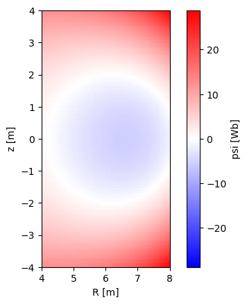
import matplotlib.pyplot as plt

psi, rho = a5.input_eval(6.2, 0, 0, 0, "psi", "rho")
print("psi = %.2f, rho = %.2f" % (psi, rho))

ax = plt.figure().add_subplot(1,1,1)
a5.input_plotrz(np.linspace(4,8,50), np.linspace(-4, 4, 100), "psi", axes=ax)
plt.show(block=False)

a5.input_free(bfield=True) # Deallocates just the magnetic field input
a5.input_free()            # Deallocates all inputs (except markers and options)

psi = -5.15, rho = 0.22

/tmp/ipykernel_4895/2993582828.py:3: AscotUnitWarning: Argument(s) r, phi, z, t given without dimensions (assumed m, degree, m, s)
  psi, rho = a5.input_eval(6.2, 0, 0, 0, "psi", "rho")
/tmp/ipykernel_4895/2993582828.py:4: DeprecationWarning: Conversion of an array with ndim > 0 to a scalar is deprecated, and will error in future. Ensure you extract a single element from your array before performing this operation. (Deprecated NumPy 1.25.)
  print("psi = %.2f, rho = %.2f" % (psi, rho))
/home/runner/work/ascot5/ascot5/a5py/ascotpy/__init__.py:780: AscotUnitWarning: Argument(s) r, z given without dimensions (assumed m, m)
  out = np.squeeze(self.input_eval(r, phi, z, t, qnt, grid=True)[:,0,:,0])

Input generation

ASCOT5 is modular when it comes to inputs. Several different implementations of magnetic field, electric field, etc. exist. When planning a study, check from the documentation (see a5py.ascot5io) what kind of inputs would serve you and what kind of data those need. The required data is listed in the write_hdf5 function corresponding to that input.

Once that is decided, there are two ways to proceed. Templates for different kind of inputs can be found in a5py.templates. Some of the templates import data from external sources, e.g. EQDSK, to ASCOT5 and using those is strongly recommended.

If no suitable template exists, one must generate the arguments for the write_hdf5 function themselves.

Running ascot5_main requires that all input parents (bfield, efield, plasma, wall, neutral, boozer, mhd, marker, options) have at least one input present. Some of these are actually rarely used in a simulation and for those it is sufficient to provide dummy data.

No matter how or what input is created, all is done via create_input method.

from a5py import Ascot
a5 = Ascot("ascot.h5")

# Call explicitly E_TC.write_hdf5 function that requires exyz as a parameter
a5.data.create_input("E_TC", exyz=np.array([0,0,0]), activate=True, desc="Zero electric field")

# Use template
a5.data.create_input("bfield analytical iter circular")

'B_GS_1185935987'

Post-processing

Simulations are post-processed by using the corresponding run group in data. Run groups provide access to the data, supports evaluation of quantities derived from the data, and host many routines to export or plot the data.

from a5py import Ascot
a5 = Ascot("ascot.h5")

# Get final (R,z) coordinates of all markers that hit the wall
r,z = a5.data.active.getstate("r", "z", state="end", endcond="wall", ids=None)

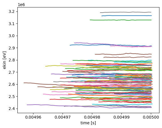
# Plot (time, energy) of confined marker orbits
ax = plt.figure().add_subplot(1,1,1)
a5.data.active.plotorbit_trajectory("time", "ekin", endcond="not wall", axes=ax)
plt.show(block=False)

# Summarize simulation
a5.data.active.getstate_markersummary()

# Visualize losses

# Etc... see the documentation of RunGroup for details

([(98, 'TLIM'), (2, 'WALL')], [])

Live simulations

The Python interface to libascot.so provides a way to run simulations directly from Python. These “live” simulations are equivalent to those run via ascot5_main except that the markers, options, and results are not stored in the HDF5 file. These simulations are convenient to use, but the main intention is to use them for post-processing or light simulations on a desktop.

Running live simulations requires that you have the inputs (excluding markers and options) present in the HDF5 file.

from a5py import Ascot
a5 = Ascot("ascot.h5")

# This method initializes and "packs" inputs in a single array. No input data can be freed while the
# data is packed.
a5.simulation_initinputs()

# Marker input can be anything but here we just use the on ascot.h5
mrk = a5.data.marker.active.read()
a5.simulation_initmarkers(**mrk)

# Options input can also be anything but here we just use the on ascot.h5
opt = a5.data.options.active.read()
a5.simulation_initoptions(**opt)

print("Input initialized")

/home/runner/work/ascot5/ascot5/a5py/ascotpy/libsimulate.py:240: AscotUnitWarning: Argument(s) r, phi, z, time, mass, charge, energy, zeta given without dimensions (assumed m, degree, m, s, amu, e, eV, rad)
  r, phi, z, t, m, q, energy, pitch, zeta, anum, znum, w, ids = parse(

Input initialized

Running the live simulation returns a VirtualRun object which in many ways behaves similarly as the RunGroup introduced earlier.

vrun = a5.simulation_run()

# Get final (R,z) coordinates of all markers that hit the wall
r, z = vrun.getstate("r", "z", state="end", endcond="wall", ids=None)
print(r,z)

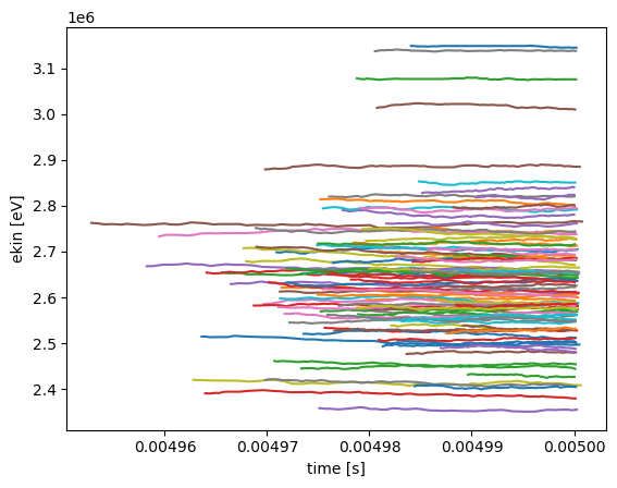
# Plot (time, energy) of confined marker orbits
ax = plt.figure().add_subplot(1,1,1)
vrun.plotorbit_trajectory("time", "ekin", endcond="not wall", axes=ax)
plt.show(block=True)

# Summarize simulation
vrun.getstate_markersummary()

# Visualize losses

# Etc... see the documentation of RunGroup for details

[4.09930708 8.41494004] m [0.29590355 0.15543651] m

([(98, 'TLIM'), (2, 'WALL')], [])

To rerun the code, free the simulation output. Once it is freed, the previous VirtualRun becomes an empty shell and it is no longer usable. Once you have had enough fun, the markers should be freed and inputs unpacked and deallocated.

a5.simulation_free(diagnostics=True)
a5.simulation_run()

a5.simulation_free(inputs=True, markers=True, diagnostics=True)

Summary of results:
       98 markers had end condition Sim time limit
        2 markers had end condition Wall collision

          No markers were aborted.

Summary of results:
       98 markers had end condition Sim time limit
        2 markers had end condition Wall collision

          No markers were aborted.

Need help?

1. Ask in our ASCOT5 Slack channel.

2. If you have an issue to report, use the GitHub issue tracker. For bugs, state which version/branch you are using and try to provide the HDF5 file.

3. Join one of our “weekly” meetings to present your research and discuss any issues.